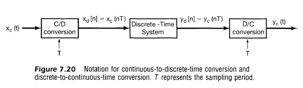
Up until now, we have focused our analysis in the continuous domain, so we will now make the transition between a sampled signal in the continuous domain (weighted impulses separated by period $T$) to the discrete domain (signal sequence for integer values of $n$).
To more easily distinguish between signal frequencies and Fourier Transforms, one can use $\omega$ in continuous time and $\Omega$ in discrete time. In other words, a signal may have frequency component $\omega$ in the time domain and $\Omega$ when sampled. $\Omega$ can be considered the “normalized” frequency relative to each sample in the discrete domain.
$T$ is the sampling period such that $\omega_s = 2 \pi / T$.

Continuous to Discrete Conversion
Recall from Time Shift Property Analysis, we can represent the Fourier Transform of a continuous time sampled signal in the $\omega$ domain as
$$
\begin{align}
x_p(t) = \sum_{n=-\infty}^{\infty} x_c(nT) \delta(t-nT) &\stackrel{\mathcal{F}}{\leftrightarrow} X_p(j \omega) = \sum_{n=-\infty}^{\infty} x_c(nT) e^{-j \omega n T} \\
\end{align}
$$
A generic discrete time signal has the Fourier Transform in the $\Omega$ domain as
$$
\begin{align}
x_d[n] &\stackrel{\mathcal{F}}{\leftrightarrow}
X_d(e^{j \Omega}) = \sum_{n=-\infty}^{\infty} x_d[n] e^{- j \Omega n} \\
\end{align}
$$
If we assert that this discrete time signal that relates to the continuous time signal by $x_d[n] = x_c(nT)$ we may rewrite the Fourier Transform as
$$
\begin{align}
x_d[n] = x_c(nT) &\stackrel{\mathcal{F}}{\leftrightarrow}
X_d(e^{j \Omega}) = \sum_{n=-\infty}^{\infty} x_c(nT) e^{- j \Omega n} \\
\end{align}
$$
Note that if we substitute the relationship $\omega = \Omega / T$ into the continuous time sampled signal $X_p(j \omega)$, we get
$$
\begin{align}
X_p(j \Omega / T) &= \sum_{n=-\infty}^{\infty} x_c(nT) e^{-j (\Omega / T) n T} &&\omega = \Omega / T \\
X_p(j \Omega / T) &= \sum_{n=-\infty}^{\infty} x_c(nT) e^{-j \Omega n} &&\omega = \Omega / T \\
\end{align}
$$
and so, the continuous and the discrete sampled cases can be compared with
$$
\begin{align}
X_d(e^{j \Omega}) = X_p(j \Omega / T) \\
\end{align}
$$
In other words, the frequency response in the continuous case at frequency $\omega$ will correspond to the discrete frequency $\Omega = \omega T$, and the resulting frequency response is scaled by $T$ in the frequency axis. This relationship $\Omega = \omega T$ is used quite frequently in subsequent analysis, and it implies the following additional relationships of note:
$$
\begin{align}
\omega &= \frac{\Omega}{T} \\
\omega &= \Omega f_s \\
2 \pi f &= \Omega f_s \\
\frac{f}{f_s} &= \frac{\Omega}{2 \pi} \\
\frac{\omega}{\omega_s} &= \frac{\Omega}{2 \pi} \\
\\
T &= \frac{\Omega}{\omega} \\
f_s &= \frac{\omega}{\Omega} \\
\end{align}
$$
Comparing Continuous and Sampled Discrete Frequency Response
Recall from the Multiplication Property Analysis that the continuous sampled signal can also be represented as a the scaled frequency response copied every $\omega_s$, and defined by
$$
\begin{align}
x_p(t) = \sum_{n=-\infty}^{\infty} x_c(nT) \delta(t-nT) &\stackrel{\mathcal{F}}{\leftrightarrow} X_p(j \omega) = \frac{1}{T} \sum_{k=-\infty}^{\infty} X_c(j(\omega – k \omega_s)) \\
\end{align}
$$
Using the substitution $\omega = \Omega / T$ we can also rewrite the frequency response as
$$
\begin{align}
X_p(j \Omega / T) = \frac{1}{T} \sum_{k=-\infty}^{\infty} X_c\left( j \left(\frac{\Omega}{T} – k \omega_s \right) \right) \\
\end{align}
$$
which we just found to be equivalent to $X_d(e^{j \Omega})$ or
$$
\begin{align}
X_d(e^{j \Omega}) &= \frac{1}{T} \sum_{k=-\infty}^{\infty} X_c\left( j \left(\frac{\Omega}{T} – k \omega_s \right) \right) \\
X_d(e^{j \Omega}) &= \frac{1}{T} \sum_{k=-\infty}^{\infty} X_c\left( j \left(\frac{\Omega}{T} – k \frac{2 \pi}{T} \right) \right) \\
X_d(e^{j \Omega}) &= \frac{1}{T} \sum_{k=-\infty}^{\infty} X_c\left( j \frac{\Omega – 2 \pi k}{T}\right) \\
\end{align}
$$
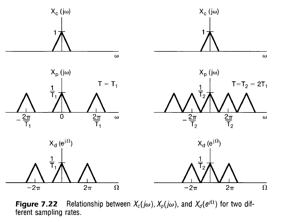
In other words, the frequency response of the discrete time sampled signal $X_d(e^{j \Omega})$ maintains the same profile as the original continuous time sampled signal with some frequency and amplitude scaling and with periodic repetition in the $\Omega$ domain.
To determine the periodicity of the frequency response, recall that in order to be periodic, the function must satisfy
$$
\begin{align}
\forall \Omega, \exists \Omega_0:&& X_d(e^{j \Omega}) &= X_d(e^{j(\Omega + \Omega_0)}) \\
&&\frac{1}{T} \sum_{k=-\infty}^{\infty} X_c\left( j \frac{\Omega – 2 \pi k}{T}\right) &= \frac{1}{T} \sum_{l=-\infty}^{\infty} X_c\left( j \frac{(\Omega + \Omega_0) – 2 \pi l}{T}\right) \\
&&\frac{\Omega – 2 \pi k}{T} &= \frac{(\Omega + \Omega_0) – 2 \pi l}{T} \\
&&\Omega – 2 \pi k &= \Omega + \Omega_0 – 2 \pi l \\
&&\Omega_0 &= 2 \pi (l – k)
\end{align}
$$
Because $l,k \in \mathbb{Z}$, the period in the $\Omega$ domain is $2 \pi$. This matches our expectations for discrete signals. In summary, sampling a signal in the continuous time and representing it in discrete time is represented by the transform
$$
\begin{align}
x_d[n] = x_c(nT) &\stackrel{\mathcal{F}}{\leftrightarrow}
X_d(e^{j \Omega}) = \frac{1}{T} \sum_{k=-\infty}^{\infty} X_c\left( j \frac{\Omega – 2 \pi k}{T}\right) \\
\end{align}
$$
Impulse Invariance: Continuous to Discrete Time System Equivalence
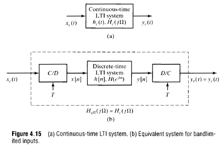
If the impulse response of a continuous time system is sampled, the discrete impulse response is represented by
$$
\begin{align}
h_d[n] = h_c(nT) &\stackrel{\mathcal{F}}{\leftrightarrow} H_d(e^{j \Omega}) = \frac{1}{T} \sum_{k=-\infty}^{\infty} H_c\left( j \frac{\Omega – 2 \pi k}{T}\right) \\
\end{align}
$$
so that the system output is
$$
\begin{align}
y_d[n] &\stackrel{\mathcal{F}}{\leftrightarrow} Y_d(e^{j \Omega}) = H_d (e^{j \Omega}) X_d(e^{j \Omega}) \\
y_d[n] &\stackrel{\mathcal{F}}{\leftrightarrow} Y_d(e^{j \Omega}) = H_d (e^{j \Omega}) \left[ \frac{1}{T} \sum_{k=-\infty}^{\infty} X_c\left( j \frac{\Omega – 2 \pi k}{T}\right) \right] \\
y_d[n] &\stackrel{\mathcal{F}}{\leftrightarrow} Y_d(e^{j \Omega}) = \frac{1}{T} \sum_{k=-\infty}^{\infty} H_d (e^{j \Omega}) X_c\left( j \frac{\Omega – 2 \pi k}{T}\right) \\
\end{align}
$$
Note that if we were to scale the sampled impulse response by $T$ to generate a new discrete system $h[n]$, we would have
$$
\begin{align}
h[n] = T h_d[n] = T h_c(nT) &\stackrel{\mathcal{F}}{\leftrightarrow} H(e^{j \Omega}) = T H_d(e^{j \Omega}) = \sum_{k=-\infty}^{\infty} H_c\left( j \frac{\Omega – 2 \pi k}{T}\right) \\
\end{align}
$$
which eliminates the scaling factor in the discrete output
$$
\begin{align}
y_d[n] &\stackrel{\mathcal{F}}{\leftrightarrow} Y_d(e^{j \Omega}) = H (e^{j \Omega}) X_d(e^{j \Omega}) \\
y_d[n] &\stackrel{\mathcal{F}}{\leftrightarrow} Y_d(e^{j \Omega}) = \frac{1}{T} \sum_{k=-\infty}^{\infty} H (e^{j \Omega}) X_c\left( j \frac{\Omega – 2 \pi k}{T}\right) \\
y_d[n] &\stackrel{\mathcal{F}}{\leftrightarrow} Y_d(e^{j \Omega}) = \frac{1}{T} \sum_{k=-\infty}^{\infty} T H_d (e^{j \Omega}) X_c\left( j \frac{\Omega – 2 \pi k}{T}\right) \\
y_d[n] &\stackrel{\mathcal{F}}{\leftrightarrow} Y_d(e^{j \Omega}) = \sum_{k=-\infty}^{\infty} H_d (e^{j \Omega}) X_c\left( j \frac{\Omega – 2 \pi k}{T}\right) \\
\end{align}
$$
Assuming we are only concerned with $|\Omega| < \pi \implies k = 0$
$$
\begin{align}
y_d[n] &\stackrel{\mathcal{F}}{\leftrightarrow} Y_d(e^{j \Omega}) = H_d (e^{j \Omega}) X_c \left( j \frac{\Omega}{T}\right) \\
\end{align}
$$
which appears very similar to the LTI output (convolving impulse response leads to pure multiplication in the frequency domain).
The method of scaling the impulse response to emulate a desired continuous time filter is known as impulse invariance. In other words, when
$$
\begin{align}
h[n] = T h_c(nT)
\end{align}
$$
then $h[n]$ is said to be an impulse invariant version of $h_c(t)$.
Examples
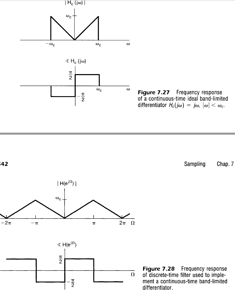
Ideal Differentiator
Recall that when attempting to design a discrete system that functions like a differentiator in continuous time, we found that the system response of
$$
\begin{align}
H(e^{j \omega}) = j \Omega \\
\end{align}
$$
is achieved with an impulse response of
$$
h[n] = \cases{
\begin{align}
0 &&&n=0 \\
\frac{(-1)^{n}}{n} &&&n \neq 0
\end{align}
}
$$
Now, using what we have learned about converting between continuous and discrete time systems and using the relation $\omega = \Omega / T$, we can refine our differentiator to more closely match the continuous case. That is, if the continuous system is described by
$$
\begin{align}
H_c(j \omega) &= j \omega \\
\end{align}
$$
then the equivalent discrete system is actually
$$
\begin{align}
H(e^{j \omega}) = j \frac{\Omega}{T} \\
\end{align}
$$
This form is very similar to the ideal differentiator system found earlier except it merely has a constant scaling factor applied to it, $1/T$, that is dependent on the sampling period. This scaling factor may then be propagated all the way down to the impulse response to yield the result that more closely represents an ideal differentiator
$$
h[n] = \cases{
\begin{align}
0 &&&n=0 \\
\frac{(-1)^{n}}{nT} &&&n \neq 0
\end{align}
}
$$
Ideal Lowpass Filter
From our previous study of the discrete time ideal lowpass filter, we may recall that
$$
h_d[n] = \frac{\sin( \Omega_c n)}{\pi n} \\
\stackrel{\mathcal{F}}{\leftrightarrow}
H_d(e^{j \Omega}) = \cases{
\begin{align}
1 &&&|\Omega| \leq \Omega_c \\
0 &&&\Omega_c < |\Omega| \leq \pi \\
\end{align}
}
$$
$$
h_d[n] = \frac{\Omega_c}{\pi} sinc(\Omega_c n)
\stackrel{\mathcal{F}}{\leftrightarrow}
H_d(e^{j \Omega}) = \cases{
\begin{align}
1 &&&|\Omega| \leq \Omega_c \\
0 &&&\Omega_c < |\Omega| \leq \pi \\
\end{align}
}
$$