Intent
Recall we found that an input signal $x[n]$ fed into an LTI system with impulse response $h[n]$ generates an output $y[n]$ described by the convolution operation.
$$
\begin{align}
x[n] &\rightarrow y[n] = x[n] * h[n] \\
x[n] &\rightarrow y[n] = \sum_{k=-\infty}^{\infty} x[k] h[n-k] \\
\end{align}
$$
As it can be fairly hard to conceptualize how a system will shape an input to an output using convolution in the $n$ domain, it is commonly beneficial to transform the representation into a new domain that is easier to conceptualize.
First, let’s imagine the simple case in discrete time where the input signal is merely some complex number raised to the $n$, that is
$$
\begin{align}
x[n] &= z^n &&&z \in \mathbb{C} \\
\\
y[n] &= x[n] * h[n] \\
y[n] &= h[n] * x[n] \\
y[n] &= \sum_{k=-\infty}^{\infty} h[k] x[n-k] \\
y[n] &= \sum_{k=-\infty}^{\infty} h[k] z^{n-k} \\
y[n] &= z^n \sum_{k=-\infty}^{\infty} h[k] z^{-k} \\
\end{align}
$$
The critical takeaway here is that the output is a scaled version of the input. In this sense, $z^n$ is called an “eigenfunction” and the scaling factor $\sum_{k=-\infty}^{\infty} h[k] z^{-k}$ is the “eigenvalue”. This eigenvalue is dependent on both the original eigenfunction $z$ and the system impulse response, and is commonly expressed as
$$
\begin{align}
H(z) &= \sum_{k=-\infty}^{\infty} h[k] z^{-k} \\
\\
y[n] &= H(z) z^n \\
y[n] &= H(z) x[n] \\
\end{align}
$$
Also note that the variable of summation for $H(z)$ can be changed to $n$ to better envision the calculation for the impulse response i.e. the eigenvalue may also be calculated using
$$
\begin{align}
H(z) &= \sum_{n=-\infty}^{\infty} h[n] z^{-n} \\
\end{align}
$$
Assuming an LTI system, if a new input signal is instead represented as a sum (series or integral) of $z$s, the output can be calculated as the sum of scaled $z$s. That is
$$
\begin{align}
x[n] = z^n &\rightarrow y[n] = H(z) z^n \\
x[n] = \sum_q a_q z_q^n &\rightarrow y[n] = \sum_q a_q H(z_q) z_q^n \\
\end{align}
$$
Note that the eigenvalue is dependent on $z$, so if the input is expressed as a sum of $z$s, then $H(z)$ must be calculated for each $z$.
The transformations here are all built on this principle and essentially just vary in what set of $z$s we can use to describe our input signal impulse response.
Discrete Time Fourier Series
The Discrete Time Fourier Series is a method to represent any periodic signal as a series of periodic exponentials.
Assume that a discrete signal may be represented as a series of periodic harmonics such that
$$
\begin{align}
x[n] &= \sum_k a_k e^{j k \Omega_0 n} \\
\end{align}
$$
Recall that there are only $N$ distinct harmonics due to discrete frequency periodicity. We can then represent this signal with
$$
\begin{align}
x[n] &= \sum_{k= \langle N \rangle} a_k e^{j k \Omega_0 n} \\
\end{align}
$$
We can solve for Fourier Series coefficients, $a_k$ by scaling both sides with another complex exponential and summing both sides over one period with respect to $n$.
$$
\begin{align}
x[n] e^{-j q \Omega_0 n} &= \sum_{k= \langle N \rangle } a_k e^{j k \Omega_0 n} e^{-j q \Omega_0 n} \\
\sum_{n = \langle N \rangle} x[n] e^{-j q \Omega_0 n} &= \sum_{n = \langle N \rangle} \sum_{k= \langle N \rangle } a_k e^{j k \Omega_0 n} e^{-j q \Omega_0 n} \\
\sum_{n = \langle N \rangle} x[n] e^{-j q \Omega_0 n} &= \sum_{n = \langle N \rangle} \sum_{k= \langle N \rangle } a_k e^{j (k-q) \Omega_0 n} \\
\sum_{n = \langle N \rangle} x[n] e^{-j q \Omega_0 n} &= \sum_{k= \langle N \rangle } a_k \sum_{n = \langle N \rangle} e^{j (k-q) \Omega_0 n} \\
\end{align}
$$
From how we defined the harmonics of $x[n]$ we know that $k \in \mathbb{Z}$. Now if we further restrict our study to cases when $k – q \in \mathbb{Z} \implies q \in \mathbb{Z}$, then we may note that the rightmost summation is 0 $ \forall q, k: q \neq k$, but the exponential is 1 when $q=k$.
If we know the LHS must be nonzero, then
$$
\begin{align}
q &= k \\
\\
\sum_{n = \langle N \rangle} x[n] e^{-j q \Omega_0 n} &= \sum_{k= q} a_k \sum_{n = \langle N \rangle} 1 &&(k = q) \land (k, q \in \mathbb{Z}) \\
\sum_{n = \langle N \rangle} x[n] e^{-j q \Omega_0 n} &= a_q N &&(k = q) \land (k, q \in \mathbb{Z}) \\
a_q &= \frac{1}{N} \sum_{n = \langle N \rangle} x[n] e^{-j q \Omega_0 n} &&(k = q) \land (k, q \in \mathbb{Z})
\end{align}
$$
and then replacing $q$ with $k$ for notation consistency, we have the synthesis and analysis equations:
$$
\boxed{
\begin{align}
x[n] &= \sum_{k = \langle N \rangle} a_k e^{j k \Omega_0 n} \\
a_k &= \frac{1}{N} \sum_{n = \langle N \rangle} x[n] e^{-j k \Omega_0 n}
\end{align}
}
$$
Discrete Time Fourier Transform
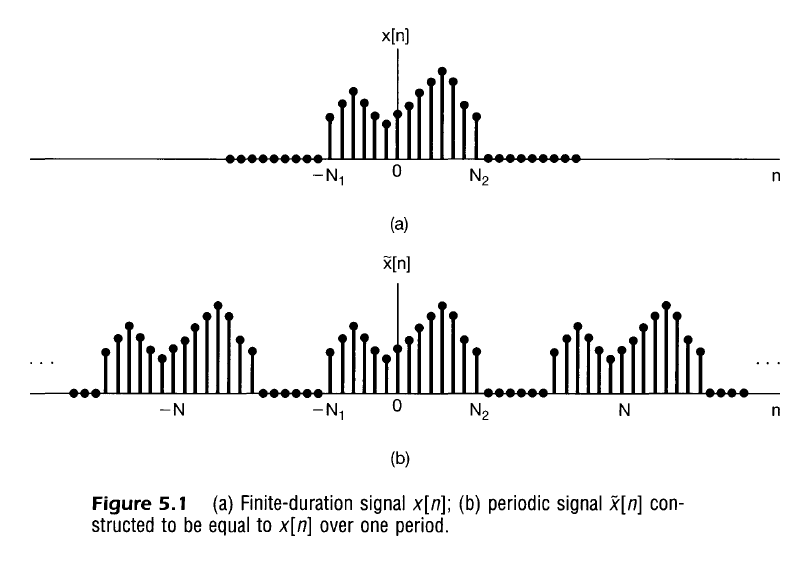
The Fourier Transform is an extension of the Fourier series that may represent finite aperiodic sequences in addition to periodic sequences.
Consider the finite duration signal $x[n]$ where $x[n] = 0$ when $-N_1 \leq n \leq N_2$. Then imagine periodic version of that signal $\tilde{x}[n]$ that repeats every $N \geq N_1 + N_2$.
Recall from the Fourier series that this periodic signal $\tilde{x}[n]$ may be represented as
$$
\begin{align}
\tilde{x}[n] &= \sum_{k=\langle N \rangle} a_k e^{j k \Omega_0 n} \\
\end{align}
$$
and so we then have Fourier Series coefficients that can be described by
$$
\begin{align}
a_k &= \frac{1}{N} \sum_{n=\langle N \rangle} \tilde{x}[n] e^{- j k \Omega_0 n} \\
a_k &= \frac{1}{N} \sum_{n=-N_2}^{N_1} \tilde{x}[n] e^{- j k \Omega_0 n} \\
a_k &= \frac{1}{N} \sum_{n=-N_2}^{N_1} x[n] e^{- j k \Omega_0 n} \\
a_k &= \frac{1}{N} \sum_{n=-\infty}^{\infty} x[n] e^{- j k \Omega_0 n} \\
\end{align}
$$
Define the “envelope function” $X$ as
$$
X(e^{j \Omega}) = \sum_{n=-\infty}^{\infty} x[n] e^{- j \Omega n} \\
$$
Using this definition of $X$ we may rewrite the Fourier Series coefficients as
$$
a_k = \frac{1}{N} X(e^{j k \Omega_0})
$$
and then the synthesis equation can be rewritten as
$$
\begin{align}
\tilde{x}[n] &= \sum_{k=\langle N \rangle} \left[ \frac{1}{N} X(e^{j k \Omega_0}) \right] e^{j k \Omega_0 n} \\
\tilde{x}[n] &= \sum_{k=\langle N \rangle} \left[ \frac{\Omega_0}{2 \pi} X(e^{j k \Omega_0}) \right] e^{j k \Omega_0 n} \\
\tilde{x}[n] &= \frac{1}{2 \pi} \sum_{k=\langle N \rangle} X(e^{j k \Omega_0}) e^{j k \Omega_0 n} \Omega_0 \\
\end{align}
$$
Now if we extend the “period” of our signal until $N \rightarrow \infty$, we essentially have a finite duration signal, and we may note the phenomena
$$
\begin{align}
\Omega_0 \rightarrow d \Omega \\
k \Omega_0 \rightarrow \Omega \\
\tilde{x} \rightarrow x \\
\end{align}
$$
So that the Analysis and Synthesis equation become, for any signal,
$$
\boxed{
\begin{align}
x[n] &= \frac{1}{2 \pi}\int_{2 \pi} X(e^{j \Omega}) e^{j \Omega n} d \Omega \\
X(e^{j \Omega}) &= \sum_{n=-\infty}^{\infty} x[n] e^{- j \Omega n} \\
\end{align}
}
$$
Note that $X$ is essentially a function of $\Omega$ and is periodic every $2 \pi$ due to the frequency periodicity of discrete signals as shown below.
$$
\begin{align}
X(e^{j (\Omega+2 \pi)}) &= \sum_{n=-\infty}^{\infty} x[n] e^{- j (\Omega+2 \pi) n} \\
X(e^{j (\Omega+2 \pi)}) &= \sum_{n=-\infty}^{\infty} x[n] e^{- j \Omega n} e^{- j \cdot 2 \pi \cdot n} \\
X(e^{j (\Omega+2 \pi)}) &= \sum_{n=-\infty}^{\infty} x[n] e^{- j \Omega n} \\ \end{align}
$$
In summary, these equations suggest that
- Any finite discrete signal (periodic or aperiodic) may be represented by a summation of complex exponentials in the frequency domain $\Omega$
- Unique complex exponentials used to describe a signal reside in a frequency range of width $2 \pi$
- The amplitude of a signal’s constituent complex exponentials are described by the function $\frac{1}{2 \pi} X(e^{j \Omega})$ which may, itself, be complex.
Z Transform
Note that for the Discrete Fourier Transform, we have been using the analysis function defined by
$$
X(e^{j \Omega})
$$
Which for any $\Omega \in \mathbb{R}$ is defined on a unit circle in the imaginary plane and repeats every $2 \pi$. If we further generalize the independent variable of this function to accept any complex input, this would be described by
$$
\begin{align}
X(r e^{j \Omega})
\end{align}
$$
This quantity is often represented by $z = r e^{j \Omega}$, and in the special case where $r=1$ we have the Fourier Transform. Re-doing the same analysis as above, but for a general complex variable $z$, we have (in “fast motion”)
$$
\begin{align}
\tilde{x}[n] &= \sum_{k= \langle N \rangle} a_k (r e^{j k \Omega_0})^n \\
\sum_{n = \langle N \rangle} \tilde{x}[n] (r e^{j q \Omega_0 })^{-n} &= \sum_{n = \langle N \rangle} \sum_{k= \langle N \rangle } a_k (r e^{j k \Omega_0 })^n (r e^{j q \Omega_0 })^{-n} \\
\sum_{n = \langle N \rangle} \tilde{x}[n] (r e^{j q \Omega_0 })^{-n} &= \sum_{n = \langle N \rangle} \sum_{k= \langle N \rangle } a_k r^n e^{j k \Omega_0 n} r^{-n} e^{-j q \Omega_0 n} \\
\sum_{n = \langle N \rangle} \tilde{x}[n] (r e^{j q \Omega_0 })^{-n} &= \sum_{n = \langle N \rangle} \sum_{k= \langle N \rangle } a_k r^{n-n} e^{j (k-q) \Omega_0 n} \\
\sum_{n = \langle N \rangle} \tilde{x}[n] (r e^{j q \Omega_0 })^{-n} &= \sum_{n = \langle N \rangle} \sum_{k= \langle N \rangle } a_k e^{j (k-q) \Omega_0 n} \\
\sum_{n = \langle N \rangle} \tilde{x}[n](r e^{j q \Omega_0 })^{-n} &= \sum_{k= \langle N \rangle } a_k \sum_{n = \langle N \rangle} e^{j (k-q) \Omega_0 n} \\
\end{align}
$$
We effectively get the same implication as before: for the kth harmonic, $k, q \in \mathbb{Z} \implies$
$$
\sum_{n = \langle N \rangle} \tilde{x}[n] (r e^{j q \Omega_0})^{-n} = \cases{
\begin{align}
\sum_{k= \langle N \rangle } a_k \sum_{n = \langle N \rangle} 1 && k = q \\
0 && k \neq q \\
\end{align}
}
$$
Assuming the LHS is nonzero, we can say
\begin{align}
\sum_{n = \langle N \rangle} \tilde{x}[n] (r e^{j q \Omega_0})^{-n} &= \sum_{k=q} a_k \sum_{n = \langle N \rangle} 1 \\
\sum_{n = \langle N \rangle} \tilde{x}[n] (r e^{j q \Omega_0})^{-n} &= a_q N \\
a_q &= \frac{1}{N} \sum_{n = \langle N \rangle} \tilde{x}[n] (r e^{j q \Omega_0})^{-n} \\
a_k &= \frac{1}{N} \sum_{n = \langle N \rangle} \tilde{x}[n] (r e^{j k \Omega_0})^{-n} \\
\end{align}
Assuming $\forall n \in \langle N \rangle, \tilde{x}[n] = x[n]$, we can expand the region of integration such that
$$
\begin{align}
a_k &= \frac{1}{N} \sum_{n=\langle N \rangle} \tilde{x}[n] (r e^{j k \Omega_0})^{-n} \\
a_k &= \frac{1}{N} \sum_{n=-\infty}^{\infty} x[n] (r e^{j k \Omega_0})^{-n} \\
\end{align}
$$
Now we define
$$
X(re^{j \Omega}) = \sum_{n=-\infty}^{\infty} x[n] (r e^{j \Omega})^{-n} \\
$$
And expanding upon our earlier findings
$$
\begin{align}
a_k &= \frac{1}{N} X(r e^{j k \Omega_0}) \\
\\
\tilde{x}[n] &= \sum_{k= \langle N \rangle} a_k (r e^{j k \Omega_0})^n \\
\tilde{x}[n] &= \sum_{k=\langle N \rangle} \left[ \frac{1}{N} X(r e^{j k \Omega_0}) \right] (r e^{j k \Omega_0})^n \\
\tilde{x}[n] &= \sum_{k=\langle N \rangle} \left[ \frac{\Omega_0}{2 \pi} X(r e^{j k \Omega_0}) \right] (r e^{j k \Omega_0})^n \\
\tilde{x}[n] &= \frac{1}{2 \pi} \sum_{k=\langle N \rangle} X(r e^{j k \Omega_0}) \cdot (r e^{j k \Omega_0})^n \Omega_0 \\
\\
N &\rightarrow \infty \\
\Omega_0 &\rightarrow d \Omega \\
k \Omega_0 &\rightarrow \Omega \\
\tilde{x} &\rightarrow x \\
\\
x[n] &= \frac{1}{2 \pi}\int_{2 \pi} X(r e^{j \Omega}) \cdot (r e^{j \Omega})^n d \Omega \\
\end{align}
$$
To put in terms of $z$, the above equation can be conceptualized as an integral along a contour with fixed $r$ and varying $\omega$ along one full counterclockwise revolution.
$$
\begin{align}
z &= r e^{j \Omega} \\
dz &= j r e^{j \Omega} d \Omega \\
dz &= j z d \Omega \\
d \Omega &= \frac{1}{j z} dz \\
\\
x[n] &= \frac{1}{2 \pi} \oint_{\Omega = \langle 2\pi \rangle} X(z) z^n \frac{1}{j z} dz \\
x[n] &= \frac{1}{2 \pi j} \oint_{\Omega = \langle 2\pi \rangle} X(z) z^{n-1} dz \\
\end{align}
$$
Integration along counterclockwise closed circular contour with fixed $r$ chosen from within ROC. As this approach is unusual, partial fraction expansion and transform tables are generally preferred. In closing, the Analysis and Synthesis equations for the z-Transform are then
$$
\boxed{
\begin{align}
X(z) &= \sum_{n=-\infty}^{\infty} x[n] z^{-n} \\
x[n] &= \frac{1}{2 \pi j} \oint_{\Omega = \langle 2\pi \rangle} X(z) z^{n-1} dz \\
\end{align}
}
$$
Note that the real part of $z$ in the analysis equation suggests that the summation does not always converge, therefore a region of Convergence or ROC must be defined for each transform.
Region of Convergence
\begin{align}
X(z) &= \sum_{n=-\infty}^{\infty} x[n] z^{-n} \\
X(r e^{j \Omega}) &= \sum_{n=-\infty}^{\infty} x[n] r^{-n} e^{-j \Omega n} \\
\end{align}
Notes:
- When $|z| = r = 1$, then we effectively get the Fourier Transform. Convergence in that case is determined solely by $x[n]$. Otherwise, convergence depends on both $x[n]$ and $r$.
- ROC must never contain poles (doesn’t converge at those locations)
- If $x[n]$ is finite duration and absolutely integrable, then the ROC is the entire $z$ plane except possibly $z=0$ and/or $z \rightarrow \infty$
- If $X(z)$ is rational, then ROC is bounded by poles, or extends to infinity.
- If the signal is right sided and circle $|z| = r_0$ is in the ROC, then $|r_1| > |r_0|$ is also in the ROC.
Note that $r_1^{-n}$ will converge faster than $r_0^{-n}$
Given a right sided signal that starts at $n=N_1$, the ROC of $z$ will include infinity when $N_1 \geq 0$ but will not include infinity when $N_1 < 0$ because then there will be some terms with positive exponent in the summation. The case when $N_1 < 0$ is further analyzed with
$$
\begin{align}
X(z) &= \sum_{n=N_1}^{\infty} x[n] z^{-n} &&N_1 < 0 \\
X(z) &= \sum_{n=N_1}^{-1} x[n] z^{-n} + \sum_{n=0}^{\infty} x[n] z^{-n} &&N_1 < 0 \\
X(z) &= \sum_{n=1}^{|N_1|} x[n] z^{n} + \sum_{n=0}^{\infty} x[n] z^{-n} &&N_1 < 0 \\
\end{align}
$$
Note that the leftmost term would then include values where $z=\infty$ would be raised to a positive number which does not converge. - If the signal is left sided and circle $|z| = r_0$ is in the ROC, then all values $0 < |z| < r_0$ are also in the ROC. ROC of $z$ will include 0 when $N_2 \leq 0$ but will not include 0 when $N_2 > 0$.
Consider the left-sided signal where the rightmost nonzero value is at $n=N_2$. The z-Transform is
$$
\begin{align}
X(z) &= \sum_{n=-\infty}^{N_2} x[n] z^{-n} \\
X(z) &= \sum_{n=-\infty}^{0} x[n] z^{-n} + \sum_{n=1}^{N_2} x[n] z^{-n} \\
\end{align}
$$
ROC does not include $r=0$ because the rightmost summation would put 0 in the denominator.