Impulse and Step Functions
$$
\delta[n] = \cases{
\begin{align}
0 &&& n \neq 0 \\
1 &&& n = 0 \\
\end{align}
}
$$
$$
u[n] = \cases{
\begin{align}
0 &&& n < 0 \\
1 &&& n \ge 0 \\
\end{align}
}
$$
Relationships of note
$$
\begin{align}
\delta[n] &= u[n] – u[n-1] \\
u[n] &= \sum_{k = -\infty}^n \delta[k] \\
\end{align}
$$
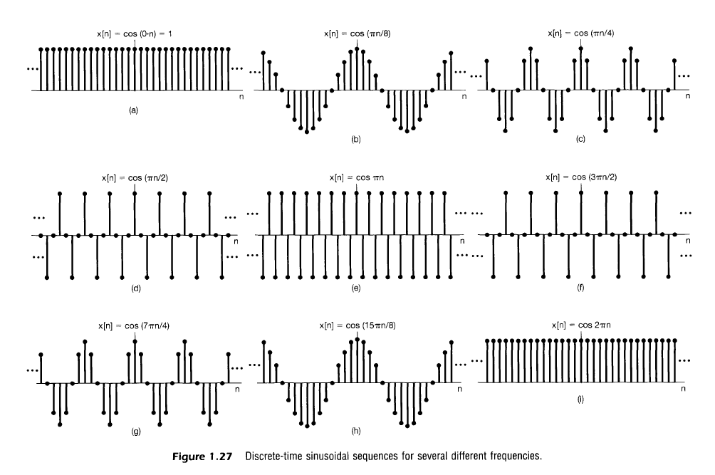
Discrete Time Frequency
\(\Omega\) represents the discrete frequency
\[
\begin{align}
\Omega &= \frac{2 \pi M}{N}
\end{align}
\]
So, the complex exponential signal
\[
\begin{align}
x[n] &= e^{j \Omega n} \\
x[n] &= e^{j (2 \pi M/N) n} \
\end{align}
\]
will oscillate \(M\) times over \(N\) discrete time steps.
Discrete Time Periodicity
For a discrete time signal \(x[n]\) to be periodic, it must satisfy
\[
\begin{align}
\forall n \in \mathbb{Z}, \exists N \in \mathbb{Z} : x[n] = x[n+N]
\end{align}
\]
Therefore, in the discrete case, we have the phenomenon where high frequency signals may appear like low frequency signals due to aliasing. This is shown by analysis of the periodic signal
\[
\begin{align}
x[n] &= x[n+N] \\
e^{j \Omega n} &= e^{j \Omega (n+N)} \\
e^{j \Omega n} &= e^{j \Omega n} e^{j \Omega N} \\
1 &= e^{j \Omega N} \\
\end{align}
\]
In order to satisfy this result, we must have
\[
\begin{align}
\Omega N = 2 \pi k &&k \in \mathbb{Z} \\
\end{align}
\]
Another way to look at this is that for a signal to be periodic in discrete time, the quantity \(\Omega / 2 \pi\) must be rational.
Discrete Frequency Periodicity
Consider complex exponential with frequency \(\Omega_1 = \Omega_0 + 2\pi\).
\[
\begin{align}
e^{j \Omega_1 n} = e^{j (\Omega_0 + 2\pi) n} \\
e^{j \Omega_1 n} = e^{j \Omega_0 n} e^{j 2 \pi n} \\
\end{align}
\]
But because \(\forall n \in \mathbb{Z}, e^{j (2\pi n)} = e^{j 2\pi} = 1\), this is simplified to
\[
e^{j \Omega_1 n} = e^{j \Omega_0 n}
\]
so effectively in discrete time signals, the discrete frequency will repeat every \(2 \pi\)
\[
\begin{align}
\Omega = \Omega_0 \pm 2\pi k &&k \in \mathbb{Z}
\end{align}
\]
Lower frequencies are near \(0\) or \(2\pi\) while higher frequencies are near \(\pm\pi\)
Sampling Property
An impulse at time $n_0$ scaled by an entire signal is equivalent to an impulse at $n_0$ scaled just by the value $x[n_0]$. That is
$$
x[n] \delta[n – n_0] = x[n_0] \delta[n – n_0]
$$
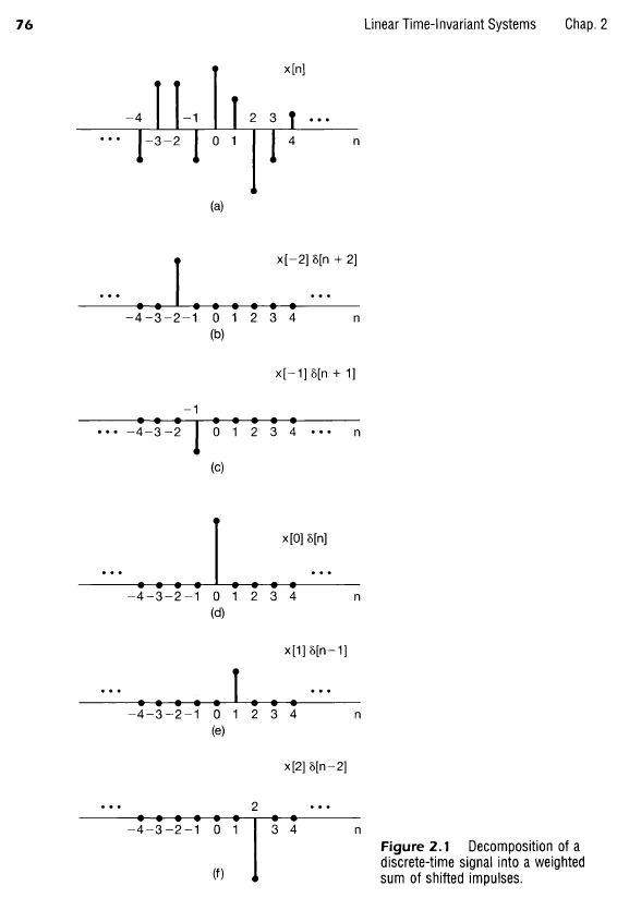
Sifting Property
The Sifting property is essentially an extension of the sampling property described above, where an alternative representation for $x[n]$ can be produced as a sum of all sampled values. In other words, a signal can be represented as a sum of unit impulses scaled by the signal at that time, $n$.
$$
\begin{align}
x[n] &= \dots + x[-2] \delta[n + 2] + x[-1] \delta[n + 1] + x[0] \delta[n] + x[1] \delta[n – 1] + x[2] \delta[n – 2] + \dots \\
x[n] &= \sum_{k = -\infty}^{\infty} x[k] \delta[n-k] \\
\end{align}
$$
Power
Power/Energy quantities tend to use squared terms
$$
\begin{align}
E_{\infty} &= \sum_{n = n_1}^{n_2} |x[n]|^2 \\
P_\infty &= \lim_{N \to \infty} \left[ \frac{1}{2N+1} \sum_{n=-N}^{N} |x[n]|^2 \right] \\
\end{align}
$$