The process described for sampling a signal is effectively reversed when going from discrete to continuous time, and we first focus on generating an idealized continuous time sampled signal (weighted pulses spaced by $T$) from the discrete time sampled signal (sequence in $n$). The continuous time sampled signal then can be fed through continuous time LPF filters that represent various real-world interpolation methods to generate the re-created signal.
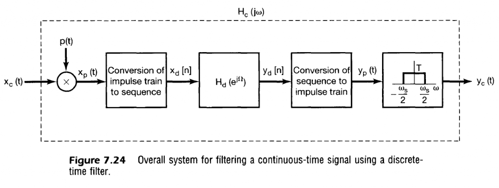
Discrete to Continuous Conversion
The impulse train can then be recreated for each discrete sample. That is
$$
\begin{align}
y_p(t) = \sum_{n=-\infty}^{\infty} y_d[n] \delta(t-nT)
&\stackrel{\mathcal{F}}{\leftrightarrow}
Y_p(j \omega) = \sum_{n=-\infty}^{\infty} y_d[n] e^{-j \omega n T} \\
\end{align}
$$
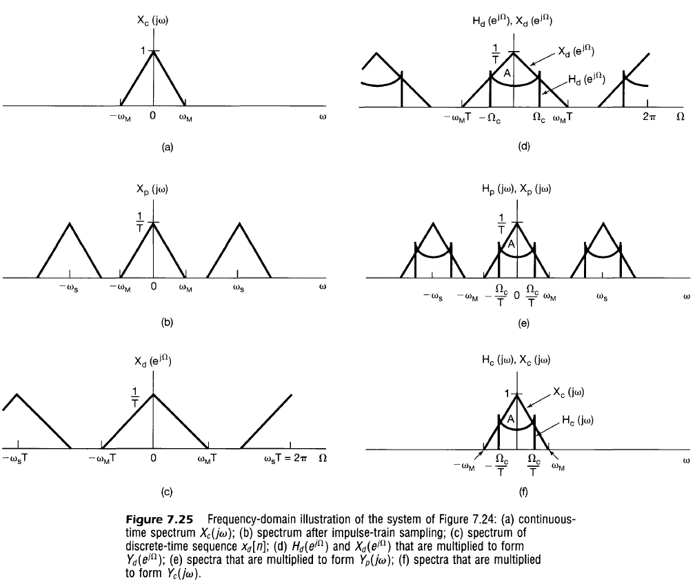
The discrete sample signal frequency response $Y_d$ will repeat every $2\pi$ in the $\Omega$ domain as any discrete signal would. We also know that the output continuous signal frequency response $Y_p(j \omega)$ will repeat in the $\omega$ domain relative to the output sampling frequency $\omega_s = 2 \pi / T$, and so $\Omega = \omega T$ still holds as a viable comparison between $\Omega$ and $\omega$ domains.
This pulsed output signal $Y_p(j \omega)$ contains information of the single desired result we want in the continuous domain, which we can denote as the idealized $Y_c$ which is repeated every $\omega_s$ in the $\omega$ domain and scaled.
$$
\begin{align}
Y_p(j \omega) &= \frac{1}{T} \sum_{k=-\infty}^{\infty} Y_c(j(\omega – k \omega_s)) \\
\end{align}
$$
From this, we can see that to accurately recreate $Y_d$ in continuous time, the ideal filter applied to $Y_p$ scales all signals $0 < |\omega| < \omega_s / 2$ by $T$, and all other frequency information is removed. This idealized interpolation method is explored further below.
Note that the following discussion reverts back to using signal $x$ instead of signal $y$ for generality.
Interpolation
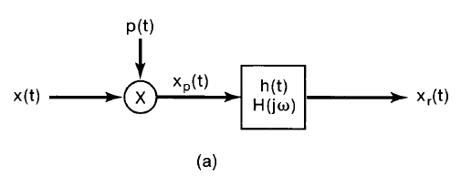
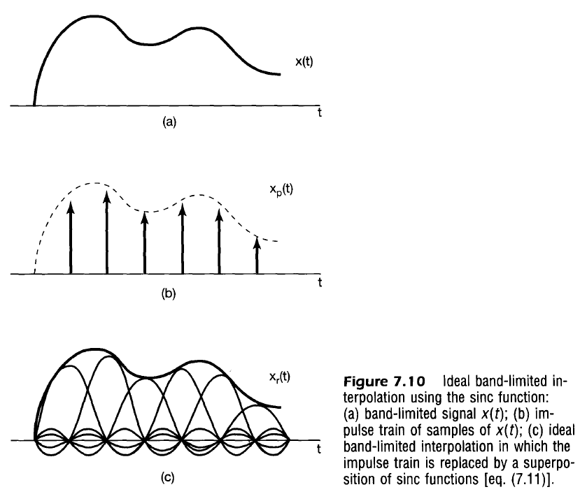
An interpolation formula describes how to fit a continuous curve between sample points $x(nT)$ using a filter $h(t) \stackrel{\mathcal{F}}{\leftrightarrow} H(j \omega)$. Note that the shape of the filter impulse response $h(t)$ is convolved with the idealized continuous sample pulse $x_p(t)$ to represent the recovered signal.
$$
\begin{align}
x_r(t) &= x_p(t) * h(t) \\
x_r(t) &= \left[ \sum_{n=-\infty}^{\infty} x(nT) \delta(t-nT) \right] * h(t) \\
x_r(t) &= \sum_{n=-\infty}^{\infty} x(nT) h(t – nT) \\
\\
X_r(j \omega) &= X_p(j \omega) H(j \omega) \\
\end{align}
$$
The analysis does not need to be limited to the idealized continuous time sampled signal, and the same result appears if using discrete sampled values and the discrete frequency response.
$$
\begin{align}
x_r(t) &= \sum_{n=-\infty}^{\infty} x_d[n] * h(t – nT) \\
\\
X_r(j \omega) &= \sum_{n=-\infty}^{\infty} x_d[n] H(j \omega) e^{-j \omega T n} \\
X_r(j \omega) &= H(j \omega) \sum_{n=-\infty}^{\infty} x_d[n] e^{-j \omega T n} \\
X_r(j \omega) &= H(j \omega) \sum_{n=-\infty}^{\infty} x_d[n] e^{-j \Omega n} \\
X_r(j \omega) &= H(j \omega) X_d(e^{j \Omega}) \\
\end{align}
$$
Ideal Signal Recreation Filter / Ideal Low-Pass Filter
This filter recreates the original signal perfectly such that $x_r(t) = x(t)$ It is difficult to implement in real-life, but provides a useful foundation of analysis.
A unity-gain low-pass filter is described by
$$
H_u(j \omega) = \cases{
\begin{align}
1 && |\omega| < \omega_c \\
0 && |\omega| \geq \omega_c \\
\end{align}
}
$$
Which can be found to have a frequency response of (TBD Reference)
$$
\begin{align}
h_u(t) &= \frac{\sin(\omega_c t)}{\pi t} \\
\end{align}
$$
Recall that the magnitude of $X_p(j \omega)$ is $X(j \omega)$ scaled by $1/T$, so in order to get the recovered signal spectrum $X_r(j \omega)$, we would need to scale the filter by the sampling period, $T$. That is, the ideal signal recovery interpolation filter is described by
$$
H(j \omega) = \cases{
\begin{align}
T && |\omega| < \omega_c \\
0 && |\omega| \geq \omega_c \\
\end{align}
}
$$
$$
\begin{align}
H(j \omega) = T H_u (j \omega)
\end{align}
$$
$$
\begin{align}
h(t) &= T \frac{\sin(\omega_c t)}{\pi t} \\
h(t) &= \frac{\omega_c T}{\pi} \frac{\sin(\omega_c t)}{\omega_c t} \\
h(t) &= \frac{\omega_c T}{\pi} sinc(\omega_c t) \\
\end{align}
$$
So the recovered signal becomes
$$
\begin{align}
x_r(t) &= \sum_{n=-\infty}^{\infty} x(nT) \frac{\omega_c T}{\pi} \frac{\sin(\omega_c (t-nT))}{\omega_c (t-nT)} \\
\end{align}
$$
In the case where we assume the signal is band-limited and no aliasing occurs, we can use $\omega_c = \omega_s/2 = \pi/T$ to get
$$
\begin{align}
h(t) &= \frac{\sin(\pi t / T)}{\pi t / T} \\
h(t) &= sinc(\pi t / T) \\
\end{align}
$$
The reconstructed signal is then described by
$$
\begin{align}
x_r(t) &= \sum_{n=-\infty}^{\infty} x(nT) h(t – nT) \\
x_r(t) &= \sum_{n=-\infty}^{\infty} x(nT) \frac{\sin[\pi (t – nT) / T]}{\pi (t – nT) / T} \\
x_r(t) &= \sum_{n=-\infty}^{\infty} x[n] \frac{\sin[\pi (t – nT) / T]}{\pi (t – nT) / T} \\
\end{align}
$$
In other words, the summation of sinc functions at each time step scaled by the original signal exactly replicates the original signal.
Zero-Order Hold
More common in practice than multiplying input signal by generated impulses. Output is equivalent to convolving $x_p(t)$ (same as above) with a filter, $H_0(j \omega)$, that has impulse response, $h_0(t)$, that is unity between $t=0$ and $t=T$.
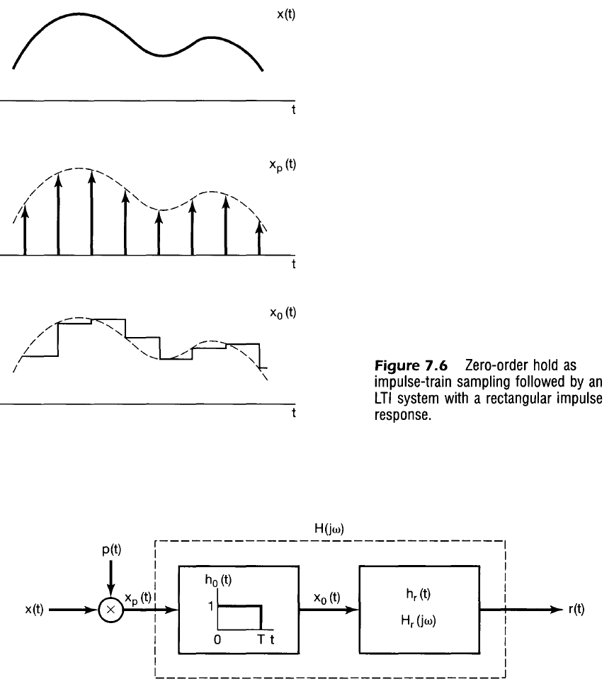
Note that $H_0(j \omega)$ is very similar to the rectangular pulse, but shifted in time.
$$
\begin{align}
H_{sq} (j \omega) &= \frac{2 sin(\omega T/2)}{\omega}
&& \text{Square of width }T\text{, centered at }t=0 \\
H_0 (j \omega) &= e^{-j \omega T/2} \frac{2 sin(\omega T/2)}{\omega}
&& \text{Square of width }T\text{, delayed by }t=T/2 \\
\end{align}
$$
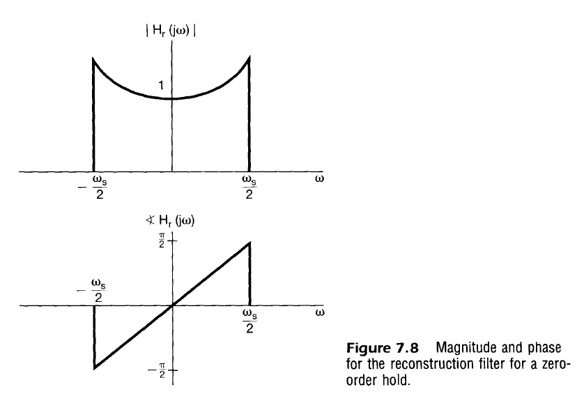
If the effects of the Zero-Order hold are desired to be reversed, an ideal reconstruction filter $H_r(j \omega)$ would be
$$
\begin{align}
H_0(j \omega) H_r(j \omega) &= 1 \\
H_r(j \omega) &= \frac{1}{H_0(j \omega)} \\
H_r(j \omega) &= \frac{1}{e^{-j \omega T/2} \frac{2 sin(\omega T/2)}{\omega}} \\
H_r(j \omega) &= \frac{e^{j \omega T/2}}{\frac{2 sin(\omega T/2)}{\omega}} \\
\end{align}
$$
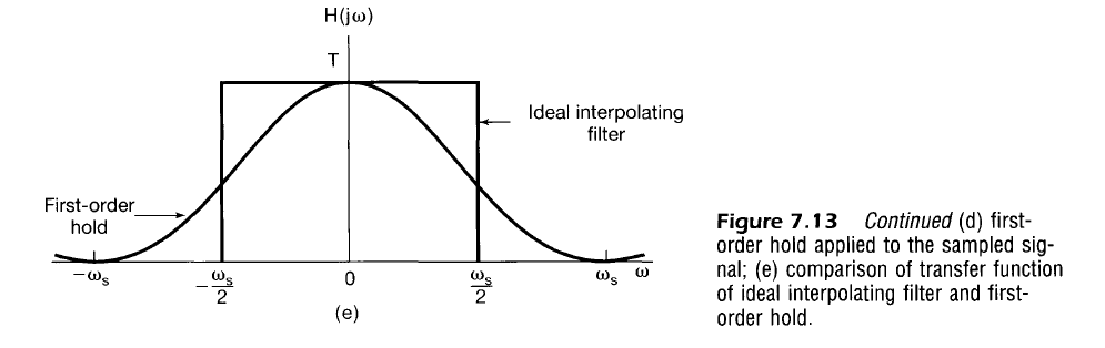
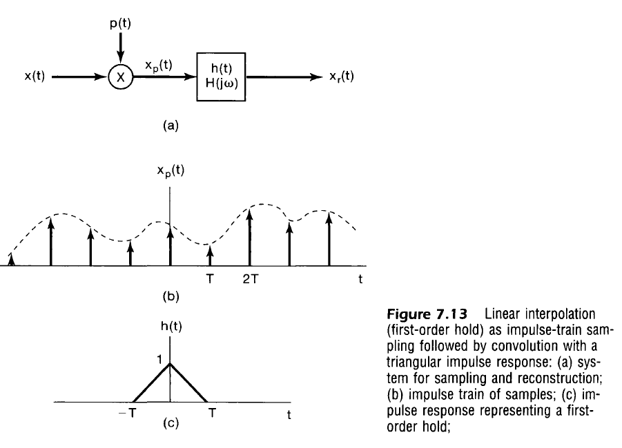
First-Order Hold/Linear Interpolation
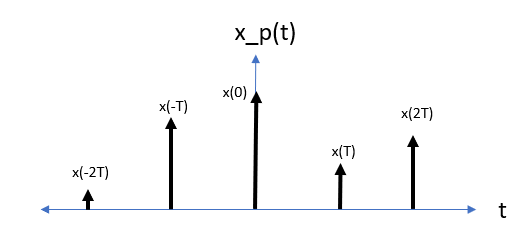
Consider $x_p(t)$, the series of impulses weighted by $x(t)$
$$
\begin{align}
x_p(t) &= \sum_{n=-\infty}^{\infty} x(nT) \delta(t-nT) \\
\end{align}
$$
An interpolating filter $h(t)$ would then generate a recreated signal, $x_r(t)$ be described as
$$
\begin{align}
x_r(t) &= x_p(t) * h(t) \\
x_r(t) &= \left[ \sum_{n=-\infty}^{\infty} x(nT) \delta(t-nT) \right] * h(t) \\
x_r(t) &= [ \cdots + x(-2T)\delta(t+2T) + x(-T)\delta(t+T) + x(0)\delta(t) + \\
&x(T)\delta(t-T) + x(2T)\delta(t-2T) + \cdots] * h(t) \\
x_r(t) &= \cdots + x(-2T)h(t+2T) + x(-T)h(t+T) + x(0)h(t) + \\
&x(T)h(t-T) + x(2T)h(t-2T) + \cdots \\
\end{align}
$$
Alternatively, one can find more simply that
$$
\begin{align}
x_r(t) &= x_p(t) * h(t) \\
x_r(t) &= \left[ \sum_{n=-\infty}^{\infty} x(nT) \delta(t-nT) \right] * h(t) \\
x_r(t) &= \sum_{n=-\infty}^{\infty} x(nT) \left[ \delta(t-nT) * h(t) \right] \\
x_r(t) &= \sum_{n=-\infty}^{\infty} x(nT) h(t-nT) \\
\end{align}
$$
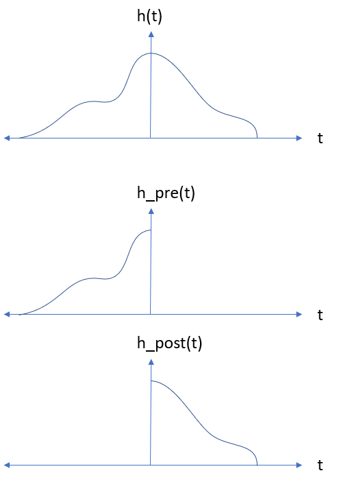
If we confine our focus to the region between two impulses of $x_p(t)$, say at some $t_0$, we can make some conceptual simplifications to determine the interpolation function. Note that in this case, all impulses of $x_p(t)$ where $t > t_0$ are weighted by the acausal side of $h(t)$ ($t < 0$) whereas all the impulses of $x_p(t)$ where $t \leq t_0$ are weighted by the causal half of $h(t)$ ($t \geq 0$). Graphically, we can split $h(t)$ into two functions where
$$ h(t) = h_{pre}(t) + h_{post}(t) $$
Now with knowledge of what we want as the output, we can define the interpolation function. For example if we know that we want
$$
\begin{align}
x_r(t_0) = x(t_0) && { t_0 | t_0=nT, n \in \mathbb{Z}} \\
\end{align}
$$
then
$$
\begin{align}
x_r(0) &= \cdots + x(-2T)h(2T) + x(-T)h(T) + x(0)h(0) + \\
&x(T)h(-T) + x(2T)h(-2T) + \cdots \\
\\
&= x(0)\\
\end{align}
$$
and
$$
\begin{align}
x_r(T) &= \cdots + x(-2T)h(T+2T) + x(-T)h(T+T) + x(0)h(T) + \\
&x(T)h(T-T) + x(2T)h(T-2T) + \cdots \\
&= \cdots + x(-2T)h(3T) + x(-T)h(2T) + x(0)h(T) + \\
&x(T)h(0) + x(2T)h(-T) + \cdots \\
&= x(T)\\
\end{align}
$$
then to be agnostic of the input function, $x(t)$, we must set
$$
\begin{align}
h(0) = 1 \\
h(t) = 0 && \forall |t| \geq T
\end{align}
$$
Now, let’s pick $t_0 \in [0,T]$ and only look at this interval. In this case we can rewrite $x_r(t)$ as
$$
\begin{align}
x_r(t_0) &= \cdots + x(-2T)h_{post}(t_0+2T) + x(-T)h_{post}(t_0+T) + x(0)h_{post}(t_0) + \\
&x(T)h_{pre}(t_0-T) + x(2T)h_{pre}(t_0-2T) + \cdots && t_0 \in [0,T] \\
\end{align}
$$
Applying these constraints, $x_r(t)$ has many terms that become 0 and it simplifies to
$$
\begin{align}
x_r(t_0) &= x(0)h_{post}(t_0) + x(T)h_{pre}(t_0-T) && t_0 \in [0,T] \\
\end{align}
$$
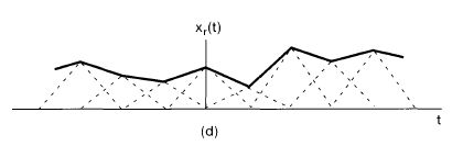
Additionally, if we want $x_r(t_0)$ to resemble a line between the two samples (first-order hold/linear interpolation), we set the equation of that line equal to $x_r(t)$ then solve for the impulse response function that makes that possible.
$$
\begin{align}
x(0)h_{post}(t_0) + x(T)h_{pre}(t_0-T) &= x(0) + \frac{x(T) – x(0)}{T} t_0 && t_0 \in [0,T] \\
x(0)h_{post}(t_0) + x(T)h_{pre}(t_0-T) &= x(0) + \frac{1}{T} x(T) t_0 – \frac{1}{T}x(0) t_0 && t_0 \in [0,T] \\
x(0)h_{post}(t_0) + x(T)h_{pre}(t_0-T) &= x(0)\left[1 – \frac{t_0}{T} \right] + x(T) \frac{t_0}{T} && t_0 \in [0,T] \\
\end{align}
$$
The impulse response function can then be isolated such that
$$
\begin{align}
h_{post}(t) = 1 – \frac{t}{T} \\
h_{post}(t) = \frac{T – t}{T} \\
\\
h_{pre}(t-T) = \frac{t}{T} \\
h_{pre}(t) = \frac{t+T}{T} \\
\end{align}
$$
and so the final impulse response is
$$
h(t) = \cases{
\begin{align}
&\frac{t+T}{T} &&-T < t < 0 \\
&\frac{T-t}{T} &&0 \leq t < T \\
&0 &&\text{Otherwise} \\
\end{align}
}
$$
Note that the impulse response is acausal, but $h(t) = 0 \;\;\; \forall t > T$, so one can effectively achieve linear interpolation with a latency of $T$.
Transfer function is determined by taking derivatives
$$
h'(t) = \cases{
\begin{align}
&\frac{1}{T} &&-T < t < 0 \\
&\frac{-1}{T} &&0 \leq t < T \\
&0 &&\text{Otherwise} \\
\end{align}
}
$$
$$
h”(t) = \frac{1}{T} \delta(t+T) – \frac{2}{T} \delta(t) + \frac{1}{T} \delta(t-T)
$$
$$
\begin{align}
H”(j \omega) = \frac{1}{T} e^{j \omega T} – \frac{2}{T} + \frac{1}{T} e^{-j \omega T} \\
H”(j \omega) = \frac{1}{T} \left[ e^{j \omega T} + e^{-j \omega T} -2 \right] \\
\end{align}
$$
$$
\begin{align}
H(j \omega) = \frac{1}{(j \omega)^2 T} \left[2 \cos(\omega T) -2 \right] &&\omega \neq 0 \\
H(j \omega) = \frac{2}{(j \omega)^2 T} \left[\cos(\omega T) – 1 \right] &&\omega \neq 0 \\
\end{align}
$$
Half Angle Formula
$$
\begin{array}{ll}
sin^2(x) = \frac{1 – cos(2x)}{2} \\
2 sin^2(x) = 1 – cos(2x) \\
cos(2x) – 1 = – 2 sin^2(x)
\end{array}
$$
$$
\begin{align}
2x = \omega T \\
x = \frac{\omega T}{2} \\
\end{align}
$$
$$
\begin{align}
H(j \omega) = \frac{2}{(j \omega)^2 T} \left[ -2 \sin^2 \left( \frac{\omega T}{2} \right) \right] &&\omega \neq 0 \\
H(j \omega) = \frac{-4 \sin^2 (\omega T/2)}{(j \omega)^2 T} &&\omega \neq 0 \\
H(j \omega) = \frac{1}{T} \frac{4 \sin^2 (\omega T/2)}{ \omega^2} &&\omega \neq 0 \\
H(j \omega) = \frac{1}{T} \frac{\sin^2 (\omega T/2)}{ (\omega / 2)^2} &&\omega \neq 0 \\
H(j \omega) = T \frac{\sin^2 (\omega T/2)}{ (\omega T / 2)^2} &&\omega \neq 0 \\
H(j \omega) = T sinc^2 (\omega T/2) &&\omega \neq 0 \\
H(j \omega) = \frac{2 \pi}{\omega_s} sinc^2 \left(\pi \frac{\omega}{\omega_s} \right) &&\omega \neq 0 \\
\end{align}
$$