Instead of differentiation used for continuous systems, discrete systems generally use difference equations to capture time-varying signal or system information.
Euler Backwards Differentiation Approximation
First Order
The Euler Backward Differentiation Approximation allows us to approximate a derivative in continuous time using discrete time samples.
$$
\begin{align}
\frac{d y(t)}{dt} &\approx \frac{y[n] – y[n-1]}{T} \\
\end{align}
$$
where $T$ is a scaling factor that represents the continuous period between samples.
Second Order
The Euler Backwards Differentiation Approximation may be further extended for second derivatives.
$$
\begin{align}
\frac{d^2 y(t)}{dt^2} &\approx \frac{ \frac{y[n] – y[n-1]}{T} – \frac{y[n-1] – y[n-2]}{T} }{ T } \\
\frac{d^2 y(t)}{dt^2} &\approx \frac{ \frac{y[n] – 2 y[n-1] + y[n-2]}{T} }{ T } \\
\frac{d^2 y(t)}{dt^2} &\approx \frac{ y[n] – 2 y[n-1] + y[n-2] }{ T^2 } \\
\end{align}
$$
$\tau / T$ and Integer Implmentation
Many of the first order systems below will express coefficients in terms of the quantity $\tau / T$ where $\tau$ is the time constant of the analagous continuous time system, and $T$ is the sampling period. This quantity may also be derived using other known quantities.
$$
\begin{align}
\frac{\tau}{T} &= \frac{1}{\omega_n T} \\
\frac{\tau}{T} &= \frac{1}{2 \pi f_n T} \\
\frac{\tau}{T} &= \frac{f_s}{2 \pi f_n} \\
\end{align}
$$
The quantity $\tau / T$ is especially useful when $\tau / T \gg 1$, and so coefficients may be generally represented using integers.
Some additional tips for using integers are:
- Apply a gain to the input signal, so the numbers used in calculation are larger
- Perform all addition and multiplication first, then apply division in one step at the end.
FIR Averaging Filter
Averaging causal FIR filter is expressed as
$$
\begin{align}
y[n] &= \frac{1}{N} \left[ x[n] + x[n-1] + \dots + x[n-(N-1)] \right] \\
\end{align}
$$
From Time Shifting Property
$$
\begin{align}
Y(z) &= \frac{1}{N} \left[ X(z) + X(z) z^{-1} + \dots + X(z) z^{-(N-1)} \right] \\
Y(z) &= \frac{1}{N} \left[ 1 + z^{-1} + \dots + z^{-(N-1)} \right] X(z) \\
\\
H(z) &= \frac{1}{N} \left[ 1 + z^{-1} + \dots + z^{-(N-1)} \right] \\
H(z) &= \frac{1}{N} \sum_{m=0}^{N-1} (z^{-1})^{m} \\
H(z) &= \frac{1}{N} \frac{1 – z^{-N}}{1 – z^{-1}} \\
\end{align}
$$
When $|z| = 1$ we get the frequency response
$$
\begin{align}
H(e^{j \Omega}) &= \frac{1}{N} \frac{1 – e^{-j \Omega N}}{1 – e^{-j \Omega}} \\
H(e^{j \Omega}) &= \frac{1}{N} \frac{e^{j \Omega / 2}}{e^{j \Omega N / 2}} \frac{e^{j \Omega N / 2}}{e^{j \Omega / 2}} \frac{1 – e^{- j \Omega N}}{1 – e^{-j \Omega}} \\
H(e^{j \Omega}) &= \frac{1}{N} \frac{e^{j \Omega / 2}}{e^{j \Omega N / 2}} \frac{e^{j \Omega N / 2} – e^{-j \Omega N / 2 }}{e^{j \Omega / 2} – e^{-j \Omega / 2}} \\
H(e^{j \Omega}) &= \frac{1}{N} \frac{e^{j \Omega / 2}}{(e^{j \Omega / 2})^N} \frac{2 j \sin( \Omega N / 2)}{2 j \sin(\Omega / 2)} \\
H(e^{j \Omega}) &= \frac{1}{N} (e^{j \Omega / 2})^{1-N} \frac{\sin( \Omega N / 2)}{\sin(\Omega / 2)} \\
\end{align}
$$
Magnitude is then
$$
\begin{align}
|H(e^{j \Omega})| &= \frac{1}{N} \left| \frac{\sin( \Omega N / 2)}{\sin(\Omega / 2)} \right| \\
\end{align}
$$
First Difference Lowpass Filter
Reference filter_algorithm.dvi (techteach.no)
Recall that in continuous time, a first order lowpass filter with some gain $G$ takes the form
$$
\begin{align}
H(s) &= G \frac{1}{\tau s + 1} \\
\\
Y(s)[\tau s + 1] &= G X(s) \\
\tau s Y(s) + Y(s) &= G X(s) \\
\\
\tau \frac{d y(t)}{dt} + y(t) &= G x(t) \\
\end{align}
$$
Using the Euler Backwards Differentiation Approximation
$$
\begin{align}
\tau \frac{y[n] – y[n-1]}{T} + y[n] &= G x[n] \\
\frac{\tau}{T} y[n] – \frac{\tau}{T} y[n-1] + y[n] &= G x[n] \\
\left( \frac{\tau}{T} + 1 \right) y[n] – \frac{\tau}{T} y[n-1] &= G x[n] \\
\end{align}
$$
Putting this in terms of a formula that may be used in an algorithm.
$$
\begin{align}
\left( \frac{\tau}{T} + 1 \right) y[n] &= \frac{\tau}{T} y[n-1] + G x[n] \\
y[n] &= \frac{ \frac{\tau}{T} y[n-1] + G x[n] }{ \frac{\tau}{T} + 1 } \\
\end{align}
$$
Frequency Response
Frequency response of this system is derived from the difference equation using $G=1$
$$
\begin{align}
\left( \frac{\tau}{T} + 1 \right) y[n] – \frac{\tau}{T} y[n-1] &= G x[n] \\
\frac{\tau + T}{T} y[n] – \frac{\tau}{T} y[n-1] &= x[n] \\
\\
\frac{\tau + T}{T} Y(e^{j \Omega}) – \frac{\tau}{T} Y(e^{j \Omega}) e^{-j \Omega} &= X(e^{j \Omega}) \\
Y(e^{j \Omega}) \left[ \frac{\tau + T}{T} – \frac{\tau}{T} e^{-j \Omega} \right] &= X(e^{j \Omega}) \\
\frac{Y(e^{j \Omega})}{X(e^{j \Omega})} &= \frac{1}{\frac{\tau + T}{T} – \frac{\tau}{T} e^{-j \Omega}} \\
H(e^{j \Omega}) &= \frac{T}{T} \frac{1}{\frac{\tau + T}{T} – \frac{\tau}{T} e^{-j \Omega}} \\
H(e^{j \Omega}) &= \frac{T}{\tau + T – \tau e^{-j \Omega}} \\
H(e^{j \Omega}) &= \frac{T}{\tau + T – \tau \cos(-\Omega) – j \tau \sin(-\Omega)} \\
H(e^{j \Omega}) &= \frac{T}{T + \tau [1 – \cos(-\Omega)] – j \tau \sin(-\Omega)} \\
H(e^{j \Omega}) &= \frac{T}{T + \tau [1 – \cos(\Omega)] + j \tau \sin(\Omega)} \\
\end{align}
$$
Magnitude is then
$$
\begin{align}
|H(e^{j \Omega})| &= \frac{T}{\sqrt{\{T + \tau [1 – \cos(\Omega)] \}^2 + \{ \tau \sin(\Omega) \}^2 } } \\
|H(e^{j \Omega})| &= \frac{T}{\sqrt{T^2 + 2 \tau T [1 – \cos(\Omega)] + \tau^2 [1 – \cos(\Omega)]^2 + \tau^2 \sin^2(\Omega) } } \\
|H(e^{j \Omega})| &= \frac{T}{\sqrt{T^2 + 2 \tau T [1 – \cos(\Omega)] + \tau^2 [1 – 2 \cos(\Omega) + \cos^2(\Omega)] + \tau^2 \sin^2(\Omega) } } \\
|H(e^{j \Omega})| &= \frac{T}{\sqrt{T^2 + 2 \tau T – 2 \tau T \cos(\Omega) + \tau^2 – 2 \tau^2 \cos(\Omega) + \tau^2 \cos^2(\Omega) + \tau^2 \sin^2(\Omega) } } \\
|H(e^{j \Omega})| &= \frac{T}{\sqrt{T^2 + 2 \tau T – 2 \tau T \cos(\Omega) + \tau^2 – 2 \tau^2 \cos(\Omega) + \tau^2 [\cos^2(\Omega) + \sin^2(\Omega)] } } \\
|H(e^{j \Omega})| &= \frac{T}{\sqrt{T^2 + 2 \tau T – 2 \tau T \cos(\Omega) + \tau^2 – 2 \tau^2 \cos(\Omega) + \tau^2 } } \\
|H(e^{j \Omega})| &= \frac{T}{\sqrt{(\tau + T)^2 – 2 \tau \cos(\Omega)(\tau + T) + \tau^2 } } \\
\end{align}
$$
There does not appear to be a simpler representation of this (when looking around on internet, trying a couple methods using sympy, and asking ChatGPT). However, you may note that if we assume the value in the radical is always positive, then the magnitude reaches a maximum when $\cos(\Omega) = 1 \implies \Omega = 0, 2 \pi, \dots$ and a minimum when $\cos(\Omega) = -1 \implies \Omega = \pm \pi, \pm 3 \pi, \dots $ as we would expect for a discrete lowpass filter.
First Difference Highpass Filter
Recall that a highpass filter in continuous time with gain $G$ is described using
$$
\begin{align}
\tau \frac{d y(t)}{dt} + y(t) &= G \tau \frac{d x(t)}{dt} \\
\end{align}
$$
Using the Euler Backwards Differentiation Approximation, we can approximate this as a difference equation in discrete time.
$$
\begin{align}
\frac{d x(t)}{dt} &\approx \frac{x[n] – x[n-1]}{T} \\
\\
\tau \frac{y[n] – y[n-1]}{T} + y[n] &= G \tau \frac{x[n] – x[n-1]}{T} \\
\frac{\tau}{T} y[n] – \frac{\tau}{T} y[n-1] + y[n] &= G \frac{\tau}{T} x[n] – G \frac{\tau}{T} x[n-1] \\
\left( \frac{\tau}{T} + 1 \right) y[n] – \frac{\tau}{T} y[n-1] &= G \frac{\tau}{T} x[n] – G \frac{\tau}{T} x[n-1] \\
\end{align}
$$
If using an algorithm, this can be rewritten
$$
\begin{align}
\left( \frac{\tau}{T} + 1 \right) y[n] &= \frac{\tau}{T} y[n-1] + G \frac{\tau}{T} x[n] – G \frac{\tau}{T} x[n-1] \\
\left( \frac{\tau}{T} + 1 \right) y[n] &= \frac{\tau}{T} \left( y[n-1] + G x[n] – G x[n-1] \right) \\
y[n] &= \frac{ ( \tau / T ) \left( y[n-1] + G \left\{ x[n] – x[n-1] \right\} \right) }{ (\tau / T ) + 1} \\
\end{align}
$$
For small changes in $x$ i.e. $x[n] – x[n-1]$ is small, one may choose the gain to be large such that
$$
\begin{align}
G &= G’ \left( \frac{\tau}{T} + 1 \right) \\
\\
\left( \frac{\tau}{T} + 1 \right) y[n] &= \frac{\tau}{T} y[n-1] + G’ \left( \frac{\tau}{T} + 1 \right) \frac{\tau}{T} x[n] – G’ \left( \frac{\tau}{T} + 1 \right) \frac{\tau}{T} x[n-1] \\
y[n] &= \frac{ \tau / T }{ ( \tau / T ) + 1 } y[n-1] + G’ \frac{\tau}{T} ( x[n] – x[n-1] ) \\
\end{align}
$$
Although the solution above does not lend itself well to an implementation, one may note that the coefficient for $y[n-1] \to 1$ whereas the $G’ (\tau / T) \gg 1$ coefficient dominates.
First Difference Differentiator
This is an easy to implement filter that resembles differentiation.
$$
\begin{align}
y[n] &= x[n] – x[n-1] \\
\\
Y(z) &= X(z) – X(z) z^{-1} \\
Y(z) &= X(z) [1 – z^{-1}] \\
H(z) &= 1 – z^{-1} \\
\\
H(e^{j \Omega}) &= 1 – e^{-j \Omega} \\
H(e^{j \Omega}) &= e^{-j \Omega/2} (e^{j \Omega/2} – e^{-j \Omega/2}) \\
H(e^{j \Omega}) &= 2 j e^{-j \Omega/2} \sin(\Omega/2) \\
\\
|H(e^{j \Omega})| &= 2 |\sin(\Omega/2)| \\
\end{align}
$$
Note around $\Omega = 0$, the magnitude is zero and slope is 1, which is similar to an ideal differentiator. Plus superscript indicates we are just looking at positive frequencies.
$$
\begin{align}
\frac{d}{d\Omega} |H(e^{j \Omega})|^+ &= 2 \cos(\Omega/2) \cdot \frac{1}{2} \\
\frac{d}{d\Omega} |H(e^{j \Omega})|^+ &= \cos(\Omega/2) \\
\left[ \frac{d}{d\Omega} |H(e^{j \Omega})| \right]_{\Omega=0^+} &= 1 \\
\end{align}
$$
Ideal Differentiator
In continuous time, a differentiating system has the form
$$
\begin{align}
y_c(t) &= \frac{d}{dt} x_c(t) \\
\end{align}
$$
And we know from the differentiation property that the system response is
$$
\begin{align}
Y_c(s) &= s X(s) \\
H_c(s) &= s \\
H_c(j \omega) &= j \omega \\
\end{align}
$$
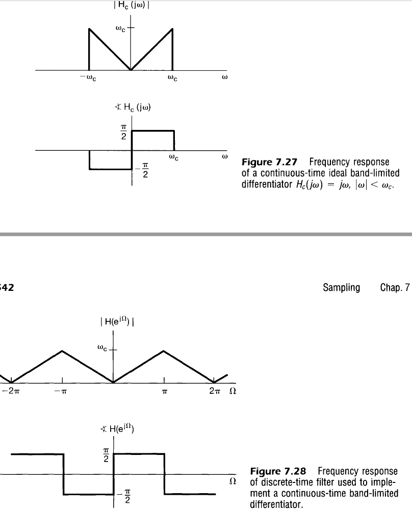
Although we will revisit this approach in more detail later, for now let’s assume that in order to create a comparable version of this filter for discrete time systems we must assume a band limited input signal and a system response described by
$$
\begin{align}
H_d(e^{j \omega}) &= j \Omega &&\left|\Omega\right| < \pi \\
\end{align}
$$
Impulse Response of this signal is
$$
\begin{align}
h_d[n] &= \frac{1}{2 \pi}\int_{2 \pi} H_d(e^{j \Omega}) \cdot e^{j \Omega n} d \Omega \\
h_d[n] &= \frac{1}{2 \pi} \int_{-\pi}^{\pi} j \Omega e^{j \Omega n} d \Omega \\
h_d[n] &= j\frac{1}{2 \pi} \int_{-\pi}^{\pi} \Omega e^{j \Omega n} d \Omega \\
\end{align}
$$
Using IBP
$$
\begin{align}
(fg)’ &= f’g + fg’ \\
f’g &= (fg)’- fg’ \\
\int_a^b f’g d\Omega &= \left[ fg \right]_{\Omega=a}^b – \int_a^b fg’ d\Omega \\
\\
f’ &= e^{j \Omega n} \\
f &= \frac{1}{j n} e^{j \Omega n} \\
g &= \Omega \\
g’ &= 1 \\
\end{align}
$$
Returning to the impulse response
$$
\begin{align}
h_d[n] &= j\frac{1}{2 \pi} \left[ \left(\frac{\Omega}{j n} e^{j \Omega n} \right)_{\Omega=-\pi}^{\pi} – \int_{-\pi}^{\pi} \frac{1}{j n} e^{j \Omega n} d \Omega \right] \\
h_d[n] &= j\frac{1}{2 \pi} \left[ \left(\frac{\Omega}{j n} e^{j \Omega n} \right)_{\Omega=-\pi}^{\pi} – \left( \frac{1}{(j n)^2} e^{j \Omega n} \right)_{\Omega=-\pi}^{\pi} \right] \\
h_d[n] &= j\frac{1}{2 \pi} \left[ \left(\frac{\pi}{j n} e^{j \pi n} – \frac{-\pi}{j n} e^{-j \pi n} \right) – \left( \frac{1}{(j n)^2} e^{j \pi n} – \frac{1}{(j n)^2} e^{-j \pi n} \right) \right] \\
h_d[n] &= j\frac{1}{2 \pi} \left[ \frac{\pi}{j n} \left( e^{j \pi n} + e^{-j \pi n} \right) – \frac{1}{(j n)^2} \left( e^{j \pi n} – e^{-j \pi n} \right) \right] \\
h_d[n] &= j\frac{1}{2 \pi} \left[ \frac{\pi}{j n} 2 \cos(\pi n) – \frac{1}{(j n)^2} 2 j \sin(\pi n) \right] \\
h_d[n] &= \frac{1}{n} \cos(\pi n) + \frac{1}{\pi (j n)^2} \sin(\pi n) \\
h_d[n] &= \frac{1}{n} \cos(\pi n) – \frac{1}{\pi n^2} \sin(\pi n) \\
h_d[n] &= \frac{\pi n \cos(\pi n) – \sin(\pi n)}{ \pi n^2} \\
\end{align}
$$
For $n \neq 0$ we may note that because $n \in \mathbb{Z}$ we can simplify the above to
$$
\begin{align}
h_d[n] &= \frac{\pi n \cos(\pi n) }{ \pi n^2} – \frac{\sin(\pi n)}{\pi n^2} &&n \neq 0 \\
h_d[n] &= \frac{\cos(\pi n) }{n} – \frac{\sin(\pi n)}{\pi n^2} &&n \neq 0 \\
n \in \mathbb{Z} \implies \sin(\pi n) = 0 \implies
h_d[n] &= \frac{\cos(\pi n) }{n} &&n \neq 0 \\
\end{align}
$$
Because both the numerator and the denominator approach 0 at $n=0$, we need to use more advanced analysis to determine the value at $n=0$. For the time being, ignore that we are solving for integer values of $n$ and instead let’s solve for the generic case where the independent variable $x \in \mathbb{R}$.
$$
\begin{align}
\frac{\pi x \cos(\pi x) – \sin(\pi x)}{ \pi x^2} \\
\end{align}
$$
Now applying L’Hôpital’s Rule just like for the $\text{sinc}$ function we get
$$
\begin{align}
\lim_{x \to c} \frac{f(x)}{g(x)} &= \lim_{x \to c} \frac{f'(x)}{g'(x)} \\
\\
f(x) &= \pi x \cos(\pi x) – \sin(\pi x) \\
\\
f'(x) &= \pi \{1 \cdot \cos(\pi x) + x \cdot [-\sin(\pi x)] \cdot \pi \} – \cos(\pi x) \cdot \pi \\
f'(x) &= \pi \{\cos(\pi x) – \pi x \sin(\pi x) \} – \pi \cos(\pi x) \\
f'(x) &= \pi \cos(\pi x) – \pi^2 x \sin(\pi x) – \pi \cos(\pi x) \\
f'(x) &= – \pi^2 x \sin(\pi x) \\
\\
g(x) &= \pi x^2 \\
\\
g'(x) &= 2 \pi x \\
\end{align}
$$
This result again cannot be solved as both the numerator and denominator approach 0 as $x \to 0$. However, we may re-use L’Hôpital’s Rule to infer that
$$
\begin{align}
\lim_{x \to c} \frac{f(x)}{g(x)} &= \lim_{x \to c} \frac{f'(x)}{g'(x)} = \lim_{x \to c} \frac{f”(x)}{g”(x)} \\
\\
f”(x) &= – \pi^2 \{ 1 \cdot \sin(\pi x) + x \cdot \cos(\pi x) \cdot \pi \} \\
f”(x) &= – \pi^2 \{ \sin(\pi x) + \pi x \cos(\pi x) \} \\
f”(x) &= – \pi^2 \sin(\pi x) – \pi^3 x \cos(\pi x) \\
\\
g”(x) &= 2 \pi \\
\end{align}
$$
The denominator no longer approaches 0, and we can now solve
$$
\begin{align}
\lim_{x \to c} \frac{f(x)}{g(x)} &= \lim_{x \to c} \frac{- \pi^2 \sin(\pi x) – \pi^3 x \cos(\pi x)}{2 \pi} \\
\lim_{x \to 0} \frac{f(x)}{g(x)} &= \lim_{x \to 0} \frac{- \pi^2 \sin(\pi x) – \pi^3 x \cos(\pi x)}{2 \pi} \\
\lim_{x \to 0} \frac{f(x)}{g(x)} &= \frac{0}{2 \pi} \\
\lim_{x \to 0} \frac{f(x)}{g(x)} &= 0 \\
\end{align}
$$
and so for the ideal differentiator in discrete time, the impulse response is
$$
h[n] = \cases{
\begin{align}
0 &&&n=0 \\
\frac{\cos(\pi n)}{n} &&&n \neq 0
\end{align}
}
$$
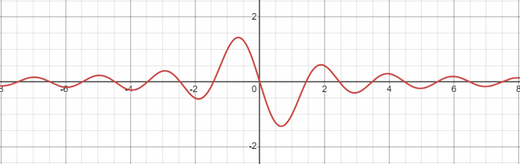
Verifying using online calculator, the continuous version of the impulse response is plotted below
$$
\begin{align}
\frac{\pi x \cos(\pi x) – \sin(\pi x)}{ \pi x^2} \\
\end{align}
$$
Below is that same plot with the discrete function superimposed over it i,e. in blue we have
$$
\begin{align}
\frac{\cos(\pi x)}{x}
\end{align}
$$
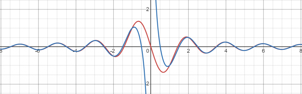
Note that the two functions overlap when $x$ is an integer except at $x=0$.
Additionally, note that $\forall n \in \mathbb{Z}$, the numerator $\cos(\pi n)$ just alternates between 1 and -1, so depending on computation method it may help to conceptualize the impulse response as
$$
h[n] = \cases{
\begin{align}
0 &&&n=0 \\
\frac{(-1)^{n}}{n} &&&n \neq 0
\end{align}
}
$$
Using the sifting property, the impulse response may also be written as
$$
\begin{align}
h[n] &= \dots +
\frac{-1}{-3} \delta[n+3] +
\frac{1}{-2} \delta[n+2] +
\frac{-1}{-1} \delta[n+1] +
0 \cdot \delta[n] +
\frac{-1}{1} \delta[n-1] +
\frac{1}{2} \delta[n-2] +
\frac{-1}{3} \delta[n-3] +
\dots \\
h[n] &= \dots +\frac{1}{3} \delta[n+3] – \frac{1}{2} \delta[n+2] +\delta[n+1] – \delta[n-1] + \frac{1}{2} \delta[n-2] – \frac{1}{3} \delta[n-3] + \dots \\
h[n] &=
(\delta[n+1] – \delta[n-1]) +
\frac{\delta[n-2] – \delta[n+2]}{2} +
\frac{\delta[n+3] – \delta[n-3]}{3} +
\dots \\
\end{align}
$$
Central Difference Differentiator
Note that if we truncate/ignore the higher order terms and can accept a latency of one sample, we have
$$
\begin{align}
h_{diffapprox}[n] &= \delta[n+1] – \delta[n-1] \\
\\
y_{diffapprox}[n] &= x[n+1] – x[n-1] \\
\\
Y_{diffapprox}(e^{j \Omega}) &= X(e^{j \Omega}) (e^{j \Omega} – e^{-j \Omega} \\
Y_{diffapprox}(e^{j \Omega}) &= X(e^{j \Omega}) 2 j \sin(\Omega) \\
H_{diffapprox}(e^{j \Omega}) &= 2 j \sin(\Omega) \\
|H_{diffapprox}(e^{j \Omega})| &= 2 \sin(\Omega) \\
\end{align}
$$
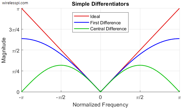
Ignoring the scaling factor of 2, this filter also resembles a differentiator at low frequencies. However, note that in this case there is some attenuation at high frequencies near $\pi$ because $\sin(\pi) = 0$. This effect is sometimes desirable however, and functions to attenuate high frequency noise and harmonics.
Reference: Design of a Discrete-Time Differentiator | Wireless Pi
Second Order Bandpass Filter
Recall that a bandpass filter in continuous time may be represented as
$$
\begin{align}
H(s) &= \frac{ s }{ s^2 + 2 \zeta \omega_n s + \omega_n^2 } \\
\end{align}
$$
Putting this in a form with derivatives using the inverse Laplace Transform, we have
$$
\begin{align}
[s^2 + 2 \zeta \omega_n s + \omega_n^2] Y(s) &= s X(s) \\
\frac{d^2 y(t)}{dt} + 2 \zeta \omega_n \frac{d y(t)}{dt} + \omega_n^2 y(t) &= \frac{d x(t)}{dt} \\
\end{align}
$$
We may then use Euler Backwards Differentiation Approximation to make a difference equation
$$
\begin{align}
\frac{ y[n] – 2 y[n-1] + y[n-2] }{ T^2 } + 2 \zeta \omega_n \left( \frac{y[n] – y[n-1]}{T} \right) + \omega_n^2 y[n] &= \frac{x[n] – x[n-1]}{T} \\
\left( \frac{1}{T^2} + \frac{ 2 \zeta \omega_n}{T} + \omega_n^2 \right) y[n] +
\left( \frac{-2}{T^2} + \frac{ -2 \zeta \omega_n}{T} \right) y[n-1] +
\frac{1}{T^2} y[n-2] &=
\frac{1}{T} x[n] +
\frac{-1}{T} x[n-1] \\
\end{align}
$$