The examples below are generally worked out for the Z Transform as it has the most generality that can be applied to the Fourier Series or the Fourier Transform. If one transform has any specific notes, it will be noted.
Convolution / LTI System
Recall that the intent of using these transforms is to make it easier to conceptualize how convolution will affect an input signal where the input signal is a sum of complex exponentials.
$$
\begin{align}
x[n] = \sum_q a_q z_q^n &\rightarrow y[n] = \sum_q a_q H(z_q) z_q^n \\
H(z) &= \sum_{n=-\infty}^{\infty} h[n] z^{-n} \\
\end{align}
$$
Fourier Series
The system eigenvalue (frequency response) is calculated from using the eigenfunction $z = e^{j k \Omega_0}$
$$
\begin{align}
H(e^{j k \Omega_0}) &= \sum_{n=-\infty}^{\infty} h[n] (e^{j k \Omega_0})^{-n} \\
H(e^{j k \Omega_0}) &= \sum_{n=-\infty}^{\infty} h[n] (e^{-j k \Omega_0 n}) \\
\\
x[n] &= \sum_{k=\langle N \rangle} a_k e^{j k \Omega_0 n} \\
\\
y[n] &= \sum_{k=\langle N \rangle} H(e^{j k \Omega_0}) a_k e^{j k \Omega_0 n} \\
\end{align}
$$
Note that the signal $y[n]$ can then be represented by a new sum
$$
\begin{align}
y[n] &= \sum_{k=\langle N \rangle} b_k e^{j k \Omega_0 n} \\
\\
b_k &= H(e^{j k \Omega_0}) a_k \\
\end{align}
$$
Note also that the Fourier Series analysis equation
$$
\begin{align}
a_k &= \frac{1}{N} \sum_{n = \langle N \rangle} x[n] e^{-j k \Omega_0 n}
\end{align}
$$
has nearly the same form as the Eigenvalue
$$
\begin{align}
H(e^{j k \Omega_0}) &= \sum_{n=-\infty}^{\infty} h[n] (e^{-j k \Omega_0 n}) \\
\end{align}
$$
but for the Fourier Series, these are not identical.
Z Transform
For the Z Transform we use the generic complex eigenfunction where $z = r e^{j \Omega}$. For LTI systems
$$
\begin{align}
H(z) &= \sum_{n=-\infty}^{\infty} h[n] z^{-n} \\
\end{align}
$$
From the synthesis equation, we found earlier we may express an input and output signal as
$$
\begin{align}
x[n] &= \frac{1}{2 \pi j} \oint_{\Omega = \langle 2\pi \rangle} X(z) z^{n-1} dz \\
y[n] &= \frac{1}{2 \pi j} \oint_{\Omega = \langle 2\pi \rangle} Y(z) z^{n-1} dz \\
\end{align}
$$
However, because the input to the system is a sum (path integral) of complex exponentials, $z$, then we can also say that the output is
$$
\begin{align}
y[n] &= \frac{1}{2 \pi j} \oint_{\Omega = \langle 2\pi \rangle} H(z) \cdot X(z) z^{n-1} dz \\
\end{align}
$$
By comparing these two equations for $y[n]$, we can better define what the scaling factor $Y(z)$ is.
$$
\begin{align}
Y(z) &= X(z) H(z) \\
\end{align}
$$
The key takeaway is that the output of a system is simply the Z Transform of the input signal multiplied by the Z Transform of the System Impulse Response. Condensing this to a more familiar form
$$
\begin{align}
x[n] &\stackrel{\mathcal{Z}}{\leftrightarrow} X(z) \\
h[n] &\stackrel{\mathcal{Z}}{\leftrightarrow} H(z) \\
y[n] = x[n] * h[n] &\stackrel{\mathcal{Z}}{\leftrightarrow} Y(z) = X(z) H(z) \\
\end{align}
$$
Another helpful takeaway is that an LTI system gain can be defined by
$$
\begin{align}
H(z) = \frac{Y(z)}{X(z)}
\end{align}
$$
The numerator of $H(z)$ contains information on the zeros of the system
The denominator of $H(z)$ contains information on the poles of the system
The magnitude and phase of $H(z)$ when $|z| = 1$ show the frequency response and phase response of the system.
Unit Impulse
Fourier Series
$$
\begin{align}
a_k &= \frac{1}{N} \sum_{n = \langle N \rangle} \delta[n] e^{-j k \Omega_0 n} \\
a_k &= \frac{1}{N} \delta[0] x[n] e^{-j k \Omega_0 \cdot 0} \\
a_k &= \frac{1}{N} \\
\end{align}
$$
Z Transform
$$
\begin{align}
x[n] &= \delta[n] \\
\\
X(z) &= \sum_{n=-\infty}^{\infty} \delta[n] z^{-n} \\
X(z) &= \delta[0] z^{0} \\
X(z) &= 1 \\
\end{align}
$$
ROC is entire $z$ plane.
Unit Step
$$
x[n] = \cases{
\begin{align}
1 &&&n \ge 0 \\
0 &&&n < 0 \\
\end{align}
}
$$
$$
\begin{align}
x[n] = u[n] \\
\\
X(z) = \sum_{n=-\infty}^{\infty} x[n] z^{-n} \\
X(z) = \sum_{n=0}^{\infty} z^{-n} \\
X(z) = \sum_{n=0}^{\infty} (z^{-1})^n \\
\end{align}
$$
Recognizing this as a geometric series
$$
\begin{align}
X(z) = \frac{1}{1 – z^{-1}} \\
\end{align}
$$
ROC is defined by
$$
\begin{align}
|z^{-1}| < 1 \\
1 < |z| \\
|z| > 1 \\
\end{align}
$$
Ideal Lowpass Filter
Fourier Transform
The ideal LPF has the following frequency response.
$$
X(e^{j \Omega}) = \cases{
\begin{align}
1 &&&|\Omega| \leq \Omega_c \\
0 &&&\Omega_c < |\Omega| \leq \pi \\
\end{align}
}
$$
From the Synthesis Equation, we can then find
$$
\begin{align}
x[n] &= \frac{1}{2 \pi}\int_{2 \pi} X(e^{j \Omega}) e^{j \Omega n} d \Omega \\
x[n] &= \frac{1}{2 \pi}\int_{-\Omega_c}^{\Omega_c} e^{j \Omega n} d \Omega \\
x[n] &= \frac{1}{2 \pi} \left[ \frac{1}{j n} e^{j \Omega n} \right]_{-\Omega_c}^{\Omega_c} \\
x[n] &= \frac{1}{2j \pi n} \left[ e^{j \Omega n} \right]_{-\Omega_c}^{\Omega_c} \\
x[n] &= \frac{1}{2j \pi n} \left[ e^{j \Omega_c n} – e^{-j \Omega_c n} \right] \\
x[n] &= \frac{1}{2j \pi n} 2 j \sin( \Omega_c n) \\
x[n] &= \frac{\sin( \Omega_c n)}{\pi n} \\
x[n] &= \frac{\Omega_c}{\pi} \frac{\sin( \Omega_c n)}{\Omega_c n} \\
x[n] &= \frac{\Omega_c}{\pi} sinc(\Omega_c n) \\
\end{align}
$$
$\sin$
Fourier Series
$$
\begin{align}
x[n] &= \sin(\Omega_0 n) \\
\end{align}
$$
Recall that the discrete frequency $\Omega_0 = \frac{2 \pi M}{N}$ so we can rewrite this signal as
$$
\begin{align}
x[n] &= \sin \left( (2 \pi M / N) n \right) \\
\end{align}
$$
which can then be decomposed into complex exponentials as
$$
\begin{align}
x[n] &= \frac{1}{2j} e^{j (2 \pi M / N) n} + \frac{-1}{2j} e^{- j (2 \pi M / N) n} \
\end{align}
$$
Comparing this result to the Synthesis equation
$$
\begin{align}
x[n] &= \sum_{k = \langle N \rangle} a_k e^{j k \Omega_{0} n} \\
\end{align}
$$
We can fit this form when
$$
\begin{align}
k \Omega_0 &= \frac{2 \pi M}{N} \\
k &= \frac{2 \pi M}{\Omega_0 N} \\
k &= M \\
\end{align}
$$
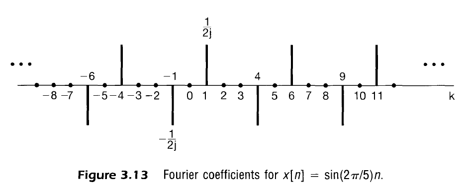
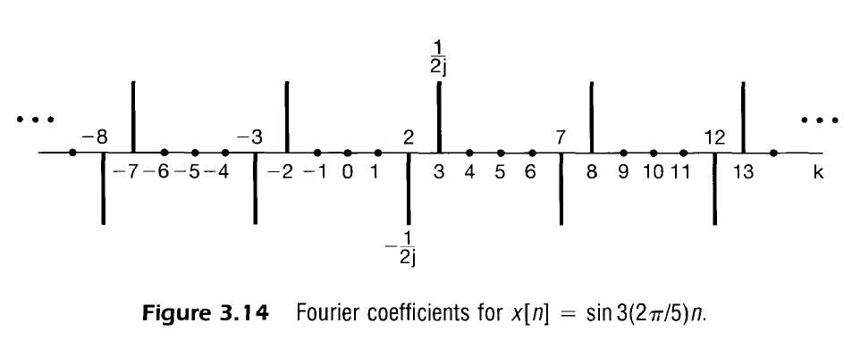
So the Fourier Series is then
$$
a_k = \cases{
\begin{align}
\frac{1}{2j} &&&k = M, M \pm N, M \pm 2N, \dots \\
\frac{-1}{2j} &&&k = -M, -M \pm N, -M \pm 2N, \dots \\
0 &&&\text{otherwise} \\
\end{align}
}
$$
In other words there is a positive spike at $k=M$ and a negative spike at $k=-M$ and that pattern repeats every $N$.
This is discussed more at length in the sampling section.
ex: $\sin(2 \pi \cdot (1/5) \cdot n)$
ex: $\sin(2 \pi \cdot (3/5) \cdot n)$
Z Transform
$$
\begin{align}
x[n] &= a^n \sin \left( \Omega_0 n \right) u[n] \\
\\
X(z) &= \sum_{n=-\infty}^{\infty} a^n \sin \left( \Omega_0 n \right) u[n] z^{-n} \\
X(z) &= \sum_{n=0}^{\infty} a^n \sin \left( \Omega_0 n \right) z^{-n} \\
X(z) &= \sum_{n=0}^{\infty} a^n \left( \frac{1}{2j} e^{j \Omega_0 n} + \frac{-1}{2j} e^{- j \Omega_0 n} \right) z^{-n} \\
X(z) &= \frac{1}{2j} \sum_{n=0}^{\infty} \left( a e^{j \Omega_0} z^{-1} \right)^n – \frac{1}{2j} \sum_{n=0}^{\infty} \left( a e^{-j \Omega_0} z^{-1} \right)^n \\
\end{align}
$$
Recalling the Geometric Series Formula
$$
\begin{align}
\sum_{i=i_1}^{i_2} r^i = \frac{r^{i_1} – r^{i_2 + 1}}{1 – r}
\end{align}
$$
Then the result
$$
\begin{align}
X(z) &= \frac{1}{2j} \frac{1}{1 – a e^{j \Omega_0} z^{-1} } – \frac{1}{2j} \frac{1}{1 – a e^{-j \Omega_0} z^{-1} } \\
X(z) &= \frac{1}{2j} \left[ \frac{1}{1 – a e^{j \Omega_0} z^{-1} } – \frac{1}{1 – a e^{-j \Omega_0} z^{-1} } \right] \\
X(z) &= \frac{1}{2j} \left[ \frac{(1 – a e^{-j \Omega_0} z^{-1}) – (1 – a e^{j \Omega_0} z^{-1}) }{(1 – a e^{j \Omega_0} z^{-1}) (1 – a e^{-j \Omega_0} z^{-1} )} \right] \\
X(z) &= \frac{1}{2j} \left[ \frac{ – a e^{-j \Omega_0} z^{-1} + a e^{j \Omega_0} z^{-1} }{(1 – a e^{j \Omega_0} z^{-1}) (1 – a e^{-j \Omega_0} z^{-1} )} \right] \\
X(z) &= a \frac{1}{2j} (e^{j \Omega_0} – e^{-j \Omega_0}) \left[ \frac{ z^{-1} }{(1 – a e^{j \Omega_0} z^{-1}) (1 – a e^{-j \Omega_0} z^{-1} )} \right] \\
X(z) &= a\sin(\Omega_0) \left[ \frac{ z^{-1} }{(1 – a e^{j \Omega_0} z^{-1}) (1 – a e^{-j \Omega_0} z^{-1} )} \right] \\
\end{align}
$$
is true when the summations converge i.e. when
$$
\begin{align}
&\lim_{n \rightarrow \infty} \left( a e^{j \Omega_0} z^{-1} \right)^n = 0 \land \lim_{n \rightarrow \infty} \left( a e^{-j \Omega_0} z^{-1} \right)^n = 0 \\
&\lim_{n \rightarrow \infty} a^n e^{j \Omega_0 n} z^{-n} = 0 \land \lim_{n \rightarrow \infty} a^n e^{-j \Omega_0 n} z^{-n} = 0 \\
&\lim_{n \rightarrow \infty} (a z^{-1})^n = 0 \\
&\left| a z^{-1} \right| < 1 \\
&|a| < |z| \\
&|z| > |a| \\
\end{align}
$$
This means that the ROC is a ring starting at radius $a$ and extending out towards infinity.
Note that the z-Transform may be rewritten in several ways. To better imagine the poles and zeros, we may write
$$
\begin{align}
X(z) &= a\sin(\Omega_0) \left[ \frac{z^2}{z^2} \frac{ z^{-1} }{(1 – a e^{j \Omega_0} z^{-1}) (1 – a e^{-j \Omega_0} z^{-1} )} \right] \\
X(z) &= a\sin(\Omega_0) \left[ \frac{ z }{(z – a e^{j \Omega_0} ) (z – a e^{-j \Omega_0} )} \right] \\
\end{align}
$$
Alternatively, if we wish to further resolve the denominator we find
$$
\begin{align}
X(z) &= a \sin(\Omega_0) \left[ \frac{ z^{-1} }{1 – a e^{j \Omega_0} z^{-1} – a e^{-j \Omega_0} z^{-1} + a^2 z^{-2} } \right] \\
X(z) &= a\sin(\Omega_0) \left[ \frac{ z^{-1} }{1 – a (e^{j \Omega_0} + e^{-j \Omega_0}) z^{-1} + a^2 z^{-2} } \right] \\
X(z) &= a\sin(\Omega_0) \left[ \frac{ z^{-1} }{1 – 2a \frac{1}{2} (e^{j \Omega_0} + e^{-j \Omega_0}) z^{-1} + a^2 z^{-2} } \right] \\
X(z) &= a\sin(\Omega_0) \left[ \frac{ z^{-1} }{1 – 2a \cos(\Omega_0) z^{-1} + a^2 z^{-2} } \right] \\
\end{align}
$$
Right-Sided Exponential
The equations below will first assume the generic signal $x[n] = a^n u[n]$. Note that this analysis will only apply to Fourier Transform and Z Transforms as the signal is inherently aperiodic.
$$
\begin{align}
x[n] &= a^n u[n] \\
\\
X(z) &= \sum_{n=-\infty}^{\infty} a^n u[n] z^{-n} \\
X(z) &= \sum_{n=0}^{\infty} a^n z^{-n} \\
X(z) &= \sum_{n=0}^{\infty} (az^{-1})^{n} \\
\end{align}
$$
Recalling the Geometric Series Formula
$$
\begin{align}
\sum_{i=i_1}^{i_2} r^i = \frac{r^{i_1} – r^{i_2 + 1}}{1 – r}
\end{align}
$$
We have
$$
\begin{align}
X(z) &= \frac{1}{1-az^{-1}} &&ROC: |az^{-1}| < 1 \\
X(z) &= \frac{z}{z-a} &&ROC: |z| > |a| \\
\end{align}
$$
Time Shifting Property
Fourier Series
$$
\begin{align}
x[n] &= \sum_{k = \langle N \rangle} a_k e^{j k \Omega_0 n} \\
\\
x[n-n_0] &= \sum_{k = \langle N \rangle} a_k e^{j k \Omega_0 (n-n_0)} \\
x[n-n_0] &= \sum_{k = \langle N \rangle} (e^{-j k \Omega_0 n_0} a_k) e^{j k \Omega_0 n} \\
\\
x[n] &\stackrel{\mathcal{FS}}{\leftrightarrow} a_k \\
x[n-n_0] &\stackrel{\mathcal{FS}}{\leftrightarrow} e^{-j k \Omega_0 n_0} a_k \\
\end{align}
$$
Fourier Transform
$$
\begin{align}
x[n] &= \frac{1}{2 \pi}\int_{2 \pi} X(e^{j \Omega}) e^{j \Omega n} d \Omega \
\\
x[n-n_0] &= \frac{1}{2 \pi}\int_{2 \pi} X(e^{j \Omega}) e^{j \Omega (n-n_0)} d \Omega \\
x[n-n_0] &= \frac{1}{2 \pi}\int_{2 \pi} \left[ e^{ -j \Omega n_0} X(e^{j \Omega}) \right] e^{j \Omega n} d \Omega \\
\end{align}
$$
So in summary
$$
x[n-n_0] \stackrel{\mathcal{F}}{\leftrightarrow} e^{-j \Omega n_0} X(e^{j \Omega}) \\
$$
Z Transform
Starting from the synthesis equation in explicit $z=re^{j\Omega}$ form
$$
\begin{align}
x[n] &= \frac{1}{2 \pi}\int_{2 \pi} X(r e^{j \Omega}) (r e^{j \Omega})^n d \Omega \\
\\
x[n-n_0] &= \frac{1}{2 \pi}\int_{2 \pi} X(r e^{j \Omega}) (r e^{j \Omega})^{n-n_0} d \Omega \\
x[n-n_0] &= \frac{1}{2 \pi}\int_{2 \pi} \left[ (r e^{j \Omega})^{-n_0} X(r e^{j \Omega}) \right] (r e^{j \Omega})^{n} d \Omega \\
\end{align}
$$
So in summary
$$
\begin{align}
x[n-n_0] &\stackrel{\mathscr{Z}}{\leftrightarrow} (r e^{j \Omega})^{-n_0} X(r e^{j \Omega}) \\
x[n-n_0] &\stackrel{\mathscr{Z}}{\leftrightarrow} z^{-n_0} X(z) \\
\end{align}
$$
Note that for this result to be true, then the analysis equation must converge. In general, the ROC is the same as the pre-shifted signal, except in certain cases: recall that the ROC of a left sided or right sided signal may exclude 0 or infinity depending on where the signal starts or ends relative to $n=0$ due to summing positive numbers to infinite exponents.
Pulse/Square Wave
Fourier Series
Assume $N$ is odd for simplicity
$$
x[n] = \cases{
\begin{align}
1 &&& |n| \le N_1 \\
0 &&& N_1 <|n| \le (N-1)/2 \\
\end{align}
}
$$
We can simplify our analysis by imagining a new signal described by
$$
\begin{align}
x'[n] &= x[n] – x[n-1] \\
x'[n] &\stackrel{\mathcal{FS}}{\leftrightarrow} a_k’ \\
\end{align}
$$
From the time shifting property, we can find that
$$
\begin{align}
a_k’ = a_k – a_k e^{-j k \Omega_0} \\
a_k’ = a_k [1 – e^{-j k \Omega_0}] \\
a_k = \frac{a_k’}{1 – e^{-j k \Omega_0}} \\
\end{align}
$$
And from evaluating $x'[n]$ in the time domain (original signal subtracted by the same signal delayed by 1), we have
$$
\begin{align}
x'[n] = \delta[n+N_1] – \delta[n – (N_1 + 1)] \\
\end{align}
$$
Noting that this result is merely time shifted impulses, we can construct the Fourier Series analysis function of $x'[n]$
$$
\begin{align}
a_k’ &= \frac{1}{N} e^{j k \Omega_0 N_1} – \frac{1}{N} e^{-j k \Omega_0 (N_1 + 1)} \\
a_k’ &= \frac{1}{N} \left[ e^{j k \Omega_0 N_1} – e^{-j k \Omega_0 (N_1 + 1)} \right] \\
a_k’ &= \frac{1}{N} \left[ e^{j k \Omega_0 N_1} – e^{-j k \Omega_0 N_1} e^{-j k \Omega_0} \right] \\
a_k’ &= \frac{1}{N} (e^{j k \Omega_0/2} e^{-j k \Omega_0/2}) \left[ e^{j k \Omega_0 N_1} – e^{-j k \Omega_0 N_1} e^{-j k \Omega_0} \right] \\
a_k’ &= \frac{1}{N} e^{-j k \Omega_0/2} \left[ e^{j k \Omega_0 N_1} e^{j k \Omega_0/2} – e^{-j k \Omega_0 N_1} e^{-j k \Omega_0/2} \right] \\
a_k’ &= \frac{1}{N} e^{-j k \Omega_0/2} \left[ e^{j k \Omega_0 (N_1 + 1/2)} – e^{-j k \Omega_0 (N_1 + 1/2)} \right] \\
a_k’ &= \frac{1}{N} e^{-j k \Omega_0/2} 2 j \frac{1}{2j} \left[ e^{j k \Omega_0 (N_1 + 1/2)} – e^{-j k \Omega_0 (N_1 + 1/2)} \right] \\
a_k’ &= \frac{1}{N} e^{-j k \Omega_0/2} 2 j \sin[k \Omega_0 (N_1 + 1/2)] \\
\end{align}
$$
And so the original signal is described by
$$
\begin{align}
a_k &= \frac{1}{1 – e^{-j k \Omega_0}} a_k’ \\
a_k &= \frac{1}{1 – e^{-j k \Omega_0}} \left[ \frac{1}{N} e^{-j k \Omega_0/2} 2 j \sin[k \Omega_0 (N_1 + 1/2)] \right] \\
a_k &= \frac{1}{N} \frac{1}{e^{j k \Omega_0/2}} \frac{1}{1 – e^{-j k \Omega_0}} 2 j \sin[k \Omega_0 (N_1 + 1/2)] \\
a_k &= \frac{1}{N} \frac{1}{e^{j k \Omega_0/2} – e^{-j k \Omega_0/2}} 2 j \sin[k \Omega_0 (N_1 + 1/2)] \\
a_k &= \frac{1}{N} \frac{1/2j}{1/2j (e^{j k \Omega_0/2} – e^{-j k \Omega_0/2}) } 2 j \sin[k \Omega_0 (N_1 + 1/2)] \\
a_k &= \frac{1}{N} \frac{\sin[k \Omega_0 (N_1 + 1/2)]}{\sin(k \Omega_0 / 2)} \\
\end{align}
$$