Complex Signals
Euler Relations
General form of the Euler Relation is
$$
\begin{align}
e^{j \theta} &= \cos(\theta) + j \sin(\theta) \\
\end{align}
$$
This relation can be inverted to yield
$$
\begin{align}
e^{j(-\theta)} &= \cos(-\theta) + j \sin(-\theta) \\
e^{-j \theta} &= \cos(\theta) – j \sin(\theta) \\
\end{align}
$$
Isolating $\cos(\theta)$ we have
$$
\begin{align}
e^{j \theta} &= \cos(\theta) + j \sin(\theta) \\
e^{-j \theta} &= \cos(\theta) – j \sin(\theta) \\
\\
e^{j \theta} + e^{-j \theta} &= 2 \cos(\theta) \\
\cos(\theta) &= \frac{1}{2}\left[ e^{j\theta} + e^{-j\theta}\right] \\
\end{align}
$$
Isolating $\sin(\theta)$ we have
$$
\begin{align}
e^{j \theta} – e^{- j \theta} &= 2 j \sin(\theta) \\
\sin(\theta) &= \frac{1}{2j}\left[ e^{j\theta} – e^{-j\theta}\right] \\
\end{align}
$$
Complex Expressions
$$
\begin{align}
|C|e^{rt}e^{j\omega_0t}e^{j\phi} = \text{ampl} \cdot \text{exp growth/decay} \cdot \text{periodic} \cdot \text{phase} \\
\\
Acos(\omega_0 t + \phi) = \frac{A}{2}e^{j\phi}e^{j \omega_0 t} + \frac{A}{2}e^{-j\phi}e^{j\omega_0 t} \\
\end{align}
$$
For complex periodic functions, we have the relations
$$
\begin{align}
e^{j \omega t} &= e^{j 2 \pi f t} \\
\\
\omega_0 &= 2 \pi f_0 \\
f_0 &= \frac{\omega_0}{2 \pi} \\
\\
T_0 &= \frac{1}{f_0} \\
T_0 &= \frac{2 \pi}{|\omega_0|} \\
\omega_0 &= \frac{2\pi}{T_0} \\
\omega_0 T_0 &= 2 \pi \\
\end{align}
$$
Even/Odd
Even
$$
\begin{align}
\text{Even Signal} \implies x(-t) &= x(t) \\
\\
Ev \left\{ x(t) \right\} &= \frac{1}{2} \left[ x(t) + x(-t) \right] \\
\end{align}
$$
Odd
$$
\begin{align}
\text{Odd Signal} \implies x(-t) &= -x(t) \\
\\
Od \left\{ x(t) \right\} &= \frac{1}{2} \left[ x(t) – x(-t) \right] \\
\end{align}
$$
Note
$$
\begin{align}
x(t) &= Ev \left\{ x(t) \right\} + Od \left\{ x(t) \right\} \\
\end{align}
$$
Periodic Signals
Periodic iff
$$
\begin{align}
\forall t \exists T :x(t) &= x(t+T) \\
\end{align}
$$
Fundamental Period $T_0$ is minimum positive nonzero value of $T$ for which above equation is satisfied.
Fundamental Frequency $\omega_0$ is then defined as
$$
\begin{align}
\omega_0 = \frac{2 \pi}{T_0} \\
\end{align}
$$
Periodic complex exponentials representing the fundamental can then be written as
$$
\begin{align}
e^{j \frac{2 \pi}{T_0} t} \\
e^{j \omega_0 t} \\
\end{align}
$$
Harmonics
Harmonics are the set of harmonically related complex exponentials with fundamental frequencies that are all multiples of a single positive frequency $\omega_0$.
$$
\begin{align}
&e^{j \omega t} \text{ is periodic with Fundamental Period } T_0 \text{ and Fundamental Frequency } \omega_0 \implies \\
&e^{j \omega_0 T_0} = 1 \implies \\
&\omega_0 T_0 = 2 \pi k, k=0, \pm1, \pm2 \dots \\
\end{align}
$$
Note that a continuous complex exponential may be periodic across infinite frequencies/periods, but there is only one fundamental that defines the set of harmonics. We then define the kth harmonic as
$$
\begin{align}
\phi_k(t) = e^{j k \frac{2 \pi}{T_0} t} \\
\phi_k(t) = e^{j k \omega_0 t} \\
\end{align}
$$
Note that when $k = 0$, the harmonic is a constant.
Power
Power/Energy quantities tend to use squared terms
$$
\begin{align}
E_{\infty} &= \int_{t_1}^{t_2} |x(t)|^2 dt \\
P_{\infty} &= \lim_{T \to \infty} \left[ \frac{1}{2T} \int_{-T}^{T} |x(t)|^2 dt \right] \\
\end{align}
$$
Periodic Power
$$
\begin{align}
E_{\text{period}} = \int_{0}^{T_0} |e^{j \omega_0 t}|^2 dt \\
E_{\text{period}} = \int_{0}^{T_0} 1^2 dt \\
E_{\text{period}} = \left[ t \right]_{0}^{T_0} \\
E_{\text{period}} = T_0 \\
P_{\text{period}} = \frac{1}{T_0}E_{\text{period}} = 1 \\
\end{align}
$$
Impulse and Step Functions
$$
u(t) = \begin{cases}
\begin{align}
0 &&t < 0 \\
1 &&t > 0 \\
\end{align}
\end{cases}
$$
Note that $u(t)$ is undefined for $t=0$
Desired relationships that mirror the discrete time case
$$
\begin{align}
u(t) &= \int_{- \infty}^t \delta(\tau) d \tau \\
\delta(t) &= \frac{d u(t)}{dt} \\
\end{align}
$$
These relationships can be used to determine how to define $\delta(t)$. Start with a continuous function with real life step over time $\Delta$.
$$
\begin{align}
\delta_{\Delta}(t) = \frac{du_{\Delta}(t)}{dt}
\end{align}
$$
Note that the $\delta_{\Delta}(t)$ function has height $1/\Delta$ and width $\Delta$, so total area is 1.
$$
\delta_{\Delta}(t) =
\begin{cases}
1/\Delta &&0 \leq t < \Delta \\
0 &&\text{otherwise} \\
\end{cases}
$$
If you now take $\lim_{\Delta \to 0} \delta_{\Delta}(t)$ we get a function that is infinitely high and infinitely thin at $t=0$ with integrated area 1. This is usually represented as a vertical arrow with height 1. When the function is scaled, the arrow changes height.
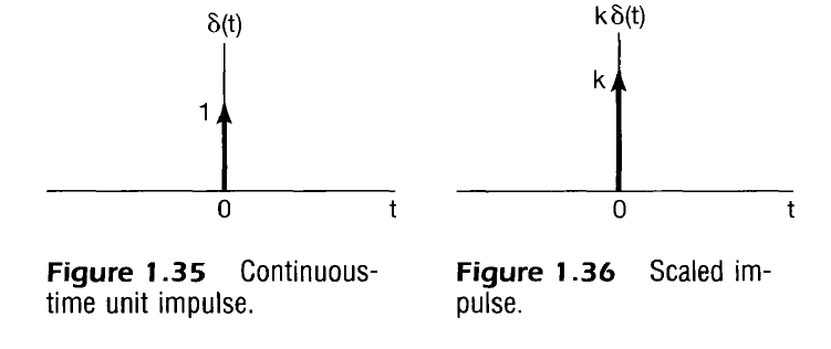
This idealized spike is then described as
$$
\begin{align}
\delta(t) = \lim_{\Delta \to 0} \delta_{\Delta}(t) \\
\end{align}
$$
Using the sifting property, we can also find that we also have the relationship
$$
\begin{align}
u(t) &= \int_{-\infty}^{\infty} u(\tau) \delta(t-\tau) d \tau \\
u(t) &= \int_{0}^{\infty} \delta(t-\tau) d \tau \\
\end{align}
$$
Sampling Property
Imagine the sample of a function $x_1(t)$ that is a function $x(t)$ multiplied by $\delta_{\Delta}(t)$, or
$$
x_1(t) = x(t) \delta_{\Delta}(t)
$$
Recalling that
$$
\delta(t) = \lim_{\Delta \rightarrow 0} \delta_{\Delta}(t)
$$
As $\Delta$ gets smaller and smaller, we can approximate $x(t)$ as constant in the interval $[0,\Delta]$, or
$$
\lim_{\Delta \rightarrow 0} x_1(t) = x(0) \delta_{\Delta}(t)
$$
Putting these properties together we get the sampling property
$$
\begin{align}
x(t) \delta(t) &= x(0) \delta(t) \\
x(t) \delta(t-t_0) &= x(t_0) \delta(t-t_0) \\
\end{align}
$$
Sifting Property
A signal may be alternatively represented as the summation (integral) of samples. This could be conceptualized as impulses across all $t$ each scaled by the original signal’s amplitude $x(t)$ at each $t$.
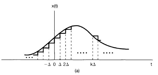
In other words, define
$$
\begin{align}
x_1(t) &=
\dots
x(-2\Delta) \delta_\Delta(t + 2\Delta) +
x(-\Delta) \delta_\Delta(t + \Delta) +
x(0) \delta_\Delta(t) +
x(\Delta) \delta_\Delta(t – \Delta) +
x(2\Delta) \delta_\Delta(t – 2\Delta) +
\dots \\
\end{align}
$$
Taking the limit as $\Delta \to 0$, the right hand side approaches an integral and the result appears closer to the original signal, so we can then say
$$
\begin{align}
x(t) &= \lim_{\Delta \to 0} x_1(t) \\
x(t) &= \lim_{\Delta \to 0} \left[
\dots
x(-2\Delta) \delta_\Delta(t + 2\Delta) +
x(-\Delta) \delta_\Delta(t + \Delta) +
x(0) \delta_\Delta(t) +
x(\Delta) \delta_\Delta(t – \Delta) +
x(2\Delta) \delta_\Delta(t – 2\Delta) +
\dots
\right] \\
x(t) &= \int_{-\infty}^{\infty} x(\tau) \delta(t – \tau) d \tau \\
\end{align}
$$