Continuous Time Sampled Signal

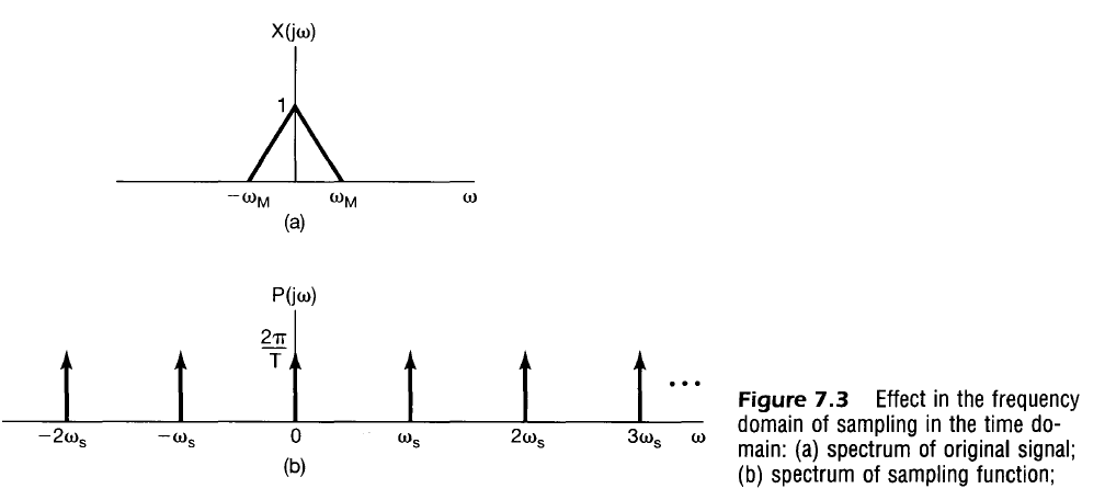
Consider the impulse train with impulses spaced $T$ sec apart.

$$
\begin{align}
p(t) &= \sum_{n=-\infty}^{\infty} \delta(t-nT) \\
\end{align}
$$

This signal then has a Sampling Frequency of $\omega_s = \frac{2 \pi}{T}$, and its Fourier Transform is (TBD on reference):

$$
\begin{align}
P(j \omega) &= \frac{2 \pi}{T} \sum_{k=-\infty}^{\infty} \delta(\omega – \frac{2 \pi k}{T}) \\
P(j \omega) &= \frac{2 \pi}{T} \sum_{k=-\infty}^{\infty} \delta(\omega – k \omega_s) \\
\end{align}
$$

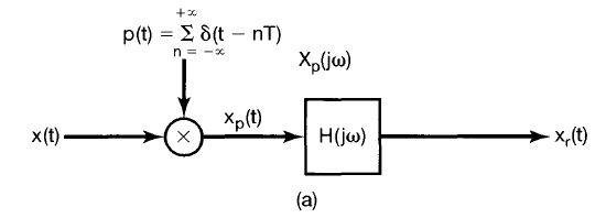
Next consider a continuous signal, $x_c(t)$ and its sampled signal $x_p(t)$ which is formed by multiplying $x_c(t)$ by the impulse train. Recalling the sampling property ($x(t) \delta(t-t_0) = x(t_0) \delta(t-t_0)$) we can say that

$$
\begin{align}
x_p(t) &= x_c(t) p(t) \\
x_p(t) &= x_c(t) \sum_{n=-\infty}^{\infty} \delta(t-nT) \\
x_p(t) &= \sum_{n=-\infty}^{\infty} x_c(t) \delta(t-nT) \\
x_p(t) &= \sum_{n=-\infty}^{\infty} x_c(nT) \delta(t-nT) \\
\end{align}
$$

Multiplication Property Analysis

From the multiplication property, the Fourier Transform of $x_p(t)$, $X_p(j \omega)$ is the convolution between $X_c(j \omega)$ and $P(j \omega)$. Because $P(j \omega)$ is merely an impulse train in the frequency domain, $X_p(j \omega)$ becomes a replication of $X_c (j \omega)$ every $\omega_s$ in the frequency domain.

$$
\begin{align}
X_p(j \omega) &= \frac{1}{2 \pi} \int_{-\infty}^{\infty} X_c(j \theta) P(j(\omega – \theta)) d \theta \\

X_p(j \omega) &= \frac{1}{2 \pi} \int_{-\infty}^{\infty} X_c(j \theta) \left[ \frac{2 \pi}{T} \sum_{k=-\infty}^{\infty} \delta(\omega – \theta – k \omega_s) \right] d \theta \\

X_p(j \omega) &= \frac{1}{T} \int_{-\infty}^{\infty} X_c(j \theta) \sum_{k=-\infty}^{\infty} \delta(\omega – \theta – k \omega_s) d \theta \\

X_p(j \omega) &= \frac{1}{T} \sum_{k=-\infty}^{\infty} \int_{-\infty}^{\infty} X_c(j \theta) \delta(\omega – \theta – k \omega_s) d \theta \\

X_p(j \omega) &= \frac{1}{T} \left[ … + \int_{-\infty}^{\infty} X_c(j \theta) \delta(\omega – \theta + \omega_s) d \theta + \int_{-\infty}^{\infty} X(j \theta) \delta(\omega – \theta) d \theta + \int_{-\infty}^{\infty} X(j \theta) \delta(\omega – \theta – \omega_s) d \theta + …\right] \\

X_p(j \omega) &= \frac{1}{T} \sum_{k=-\infty}^{\infty} X_c(j(\omega – k \omega_s)) \\

\end{align}
$$

The second to last line can be conceptualized as successive convolutions between $X(j \omega)$ and impulses each offset by $k\omega_s$and scaled by $1/T$ .

The summarized result here is that the sampled frequency response can be visualized easily from the frequency response of the continuous signal (copies every $\omega_s$).

$$
\begin{align}
x_p(t) = \sum_{n=-\infty}^{\infty} x_c(nT) \delta(t-nT)
&\stackrel{\mathcal{F}}{\leftrightarrow}
X_p(j \omega) = \frac{1}{T} \sum_{k=-\infty}^{\infty} X_c(j(\omega – k \omega_s))
\end{align}
$$

Time Shift Property Analysis

Now, consider the Continuous Fourier Transform of an impulse and modifying it in the continuous domain as shown below

$$
\begin{align}
\delta(t) &\stackrel{\mathcal{F}}{\leftrightarrow} 1 \\
\delta(t-nT) &\stackrel{\mathcal{F}}{\leftrightarrow} e^{-j \omega nT} \\
x_c(nT) \delta(t-nT) &\stackrel{\mathcal{F}}{\leftrightarrow} x_c(nT)e^{-j \omega nT} \\
\sum_{n=-\infty}^{\infty} x_c(nT) \delta(t-nT) &\stackrel{\mathcal{F}}{\leftrightarrow} \sum_{n=-\infty}^{\infty} x_c(nT)e^{-j \omega nT} \\
\end{align}
$$

Therefore, the Fourier transform of equally spaced weighted impulses can be represented by a composition of samples multiplied by corresponding phase delays.

$$
\begin{align}
x_p(t) = \sum_{n=-\infty}^{\infty} x_c(nT) \delta(t-nT)
&\stackrel{\mathcal{F}}{\leftrightarrow}
X_p(j \omega) = \sum_{n=-\infty}^{\infty} x_c(nT) e^{-j \omega n T} \\
\end{align}
$$

Nyquist Frequency

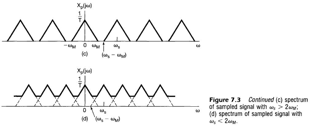
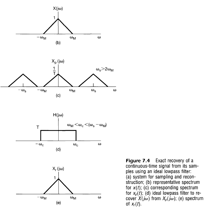
If $x(t)$ is a band-limited signal ($X(j \omega) = 0$ when $|\omega| > \omega_M$) then $x(t)$ is uniquely determined by samples iff

$$
\omega_s > 2 \omega_M =\text{Nyquist Rate} \\
$$

The original signal may be recovered from the sampled signal (frequency response curve placed every $\pm k \omega_s$) using a LPF so that only the frequency response centered at $\omega=0$ is kept.

$$

Anti-Aliasing Filter

Consider an input signal of just constant noise, that is

$$
\begin{align}
X_c(j \omega) = C \\
\end{align}
$$

Then due to the Multiplication Analysis of sampled signals, we have

$$
\begin{align}
X_p(j \omega) &= \frac{1}{T} \sum_{k=-\infty}^{\infty} X_c(j(\omega – k \omega_s)) \\
\end{align}
$$

If no low-pass filtering occurs, then the result diverges. In reality, however, there is usually at least one pole associated with sampling the input. Note that in that case we have

$$
\begin{align}
X_c(j \omega) &= C \frac{1}{1 + j \tau \omega} \\
\\
X_p(j \omega) &= \frac{1}{T} \sum_{k=-\infty}^{\infty} C \frac{1}{1 + j \tau (\omega – k \omega_s)} \\
X_p(j \omega) &= \frac{C}{T} \sum_{k=-\infty}^{\infty} \frac{1}{1 + j \tau (\omega – k \omega_s)} \\
X_p(j \omega) &= \frac{C}{T} \left[ \dots + \frac{1}{1 + j \tau (\omega + 2 \omega_s)} + \frac{1}{1 + j \tau (\omega + \omega_s)} + \frac{1}{1 + j \tau \omega} + \frac{1}{1 + j \tau (\omega – \omega_s)} + \frac{1}{1 + j \tau (\omega – 2 \omega_s)} + \dots \right] \\
\end{align}
$$

With some rearranging

$$
\begin{align}
X_p(j \omega) &= \frac{C}{T} \left[ \frac{1}{1 + j \tau \omega} + \left(\frac{1}{1 + j \tau (\omega + \omega_s)} + \frac{1}{1 + j \tau (\omega – \omega_s)} \right) + \left( \frac{1}{1 + j \tau (\omega + 2 \omega_s)} + \frac{1}{1 + j \tau (\omega – 2 \omega_s)} \right) + \dots \right] \\

X_p(j \omega) &= \frac{C}{T} \left[ \frac{1}{1 + j \tau \omega} + \sum_{k=1}^{\infty} \left(\frac{1}{1 + j \tau (\omega + k\omega_s)} + \frac{1}{1 + j \tau (\omega – k\omega_s)} \right) \right] \\

X_p(j \omega) &= \frac{C}{T} \left[ \frac{1}{1 + j \tau \omega} + \sum_{k=1}^{\infty} \frac{1 + j \tau (\omega – k\omega_s) + 1 + j \tau (\omega + k\omega_s)}{[1 + j \tau (\omega + k\omega_s)] [1 + j \tau (\omega – k\omega_s)]} \right] \\

X_p(j \omega) &= \frac{C}{T} \left[ \frac{1}{1 + j \tau \omega} + \sum_{k=1}^{\infty} \frac{2 + j 2 \tau \omega}{1 + j \tau (\omega – k\omega_s) + j \tau (\omega + k\omega_s) – \tau^2(\omega^2 – k^2 \omega_s^2)} \right] \\

X_p(j \omega) &= \frac{C}{T} \left[ \frac{1}{1 + j \tau \omega} + \sum_{k=1}^{\infty} \frac{2 + j 2 \tau \omega}{1 + j 2 \tau \omega – \tau^2(\omega^2 – k^2 \omega_s^2)} \right] \\

X_p(j \omega) &= \frac{C}{T} \left[ \frac{1}{1 + j \tau \omega} + 2\sum_{k=1}^{\infty} \frac{1 + j \tau \omega}{1 + j 2 \tau \omega – \tau^2 \omega^2 – \tau^2 \omega_s^2 k^2} \right] \\

\end{align}
$$

As an aside, consider the Basel problem which has been proven (using advanced mathematical methods) to be

$$
\begin{align}
\sum_{k=1}^{\infty} \frac{1}{k^2} = \frac{\pi^2}{6}
\end{align}
$$

Note that the summation above could be rewritten in the form

$$
\begin{align}
\sum_{k=1}^{\infty} \frac{1}{a + k^2} \\
\end{align}
$$

I would like to say that the series is convergent by the comparison test

$$
\frac{1}{a + k^2} < \frac{1}{k^2}
$$

But this should be revisited with more mathematical rigor to make sure that

1. $a$ is indeed positive
2. imaginary $j$ does not impact the result.