Discrete systems can generally be represented by an input signal $x[n]$ being modified to form an output signal $y[n] = f(x[n])$
LTI Systems
LTI, or Linear Time-Invariant systems have some desirable properties which are discussed in more detail below.
Linear
Linear systems possess the superposition property. That is, for $a, b \in \mathbb{C}$ we have
$$
\begin{align}
a x_1[n] + b x_2[n] \rightarrow a y_1[n] + b y_2[n] \\
\end{align}
$$
Note that this implies $x(t) = 0 \rightarrow y(t) = 0$. This “zero-in/zero-out” property can be used to quickly prove if a system is nonlinear in some cases.
As an example, let’s examine the system described by $y(t) = t x(t)$. Summing scaled versions of $y[n]$ on the LHS:
$$
\begin{align}
a y_1[n] + b y_2[n] &= a \{t x_1[n]\} + b \{t x_2[n]\} \\
a y_1[n] + b y_2[n] &= a t x_1[n] + b tx_2[n] \\
\end{align}
$$
Now, summing scaled versions of $x[n]$ on the RHS and submitting the result as an input to the system yields
$$
\begin{align}
t\{a x_1[n] + b x_2[n]\} = a t x_1[n] + b tx_2[n] \\
\end{align}
$$
Evaluating the RHS and LHS independently yields the same result, so the system is linear.
On the other hand, we can look at the system described by $y[n] = x[n]^2$. Summing scaled versions of $y[n]$ (LHS) we have
$$
\begin{align}
a y_1[n] + b y_2[n] = a x_1[n]^2 + b x_2[n]^2 \\
\end{align}
$$
And summing scaled versions of $x[n]$ (RHS) and submitting the result as the input to the system yields
$$
\begin{align}
\{a x_1[n] + b x_2[n]\}^2 = a^2 x_1^2[n] + b^2 x_2^2[n] + 2 a b x_1[n] x_2[n] \\
\end{align}
$$
In this case, the LHS and RHS do not match, so the system is nonlinear.
Note that the linearity of a system is sometimes not intuitive. Consider $y[n] = 2 x[n] + 3$. Summing scaled versions of $y[n]$ we have
$$
\begin{align}
a y_1[n] + b y_2[n] &= a \{2 x_1[n] + 3\} + b \{2 x_2[n] + 3\} \\
a y_1[n] + b y_2[n] &= 2 a x_1[n] + 2 b x_2[n] + 3(a+b) \\
\end{align}
$$
and summing scaled versions of $x[n]$ and feeding the result as an input yields
$$
\begin{align}
2[a x_1[n] + b x_2[n]] + 3 &= 2 a x_1[n] + 2 b x_2[n] + 3 \\
\end{align}
$$
Note that the results do not match, so this system is nonlinear. Note that even though the equation is linear, the system is not. Also upon inspection, this system has a “zero-input response” of $y_0 = 3$
A simple system is represented by $y[n] = 2 x[n]$. Linear combination of $y[n]$ yields
$$
\begin{align}
a y_1[n] + b y_2[n] = a \{2 x_1[n]\} + b \{2 x_2[n]\} \\
\end{align}
$$
and linear combination of $x[n]$ as an input yields
$$
\begin{align}
2\{a x_1[n] + b x_2[n]\} = 2 a x_1[n] + 2 b x_2[n] \\
\end{align}
$$
These results do indeed match, so the system is linear.
Time Invariant
A system is Time Invariant if its characteristics remain unchanged over time. In other words, a time invariant system yields identical results if the same input is run today vs tomorrow.
More formally, if a time shift in the input signal generates an identical time shift in the output, then the system is time invariant.
$$
\begin{align}
x[n – n_0] \rightarrow y[n-n_0] \\
\end{align}
$$
Consider $y[n] = \sin(x[n])$. For easier bookkeeping, let’s define
$$
\begin{align}
y_1[n] = \sin(x_1[n]) \\
\end{align}
$$
Introducing a time shift to the input may be represented by
$$
\begin{align}
x_2[n] = x_1[n – n_0] \\
\end{align}
$$
and the output generated when $x_2$ is the input is then
$$
\begin{align}
y_2[n] &= \sin(x_2[n]) \\
y_2[n] &= \sin(x_1[n-n_0]) \\
\end{align}
$$
Alternately, if we just introduce a time shift to the original output, $y_1[n]$, we have
$$
\begin{align}
y_1[n-n_0] &= \sin(x_1[n-n_0]) \\
\end{align}
$$
which is the same as $y_2$ which was generated from a time shifted input. Thus, the time shifted output and time shifted input fed through the system yield the same result, therefore, the system is time invariant.
Now consider the system described by $y[n] = x[2n]$ that represents a time compression of the input signal $x[n]$. I originally attempted to apply some mathematical rigor to the proof, but the counterexample is much easier.
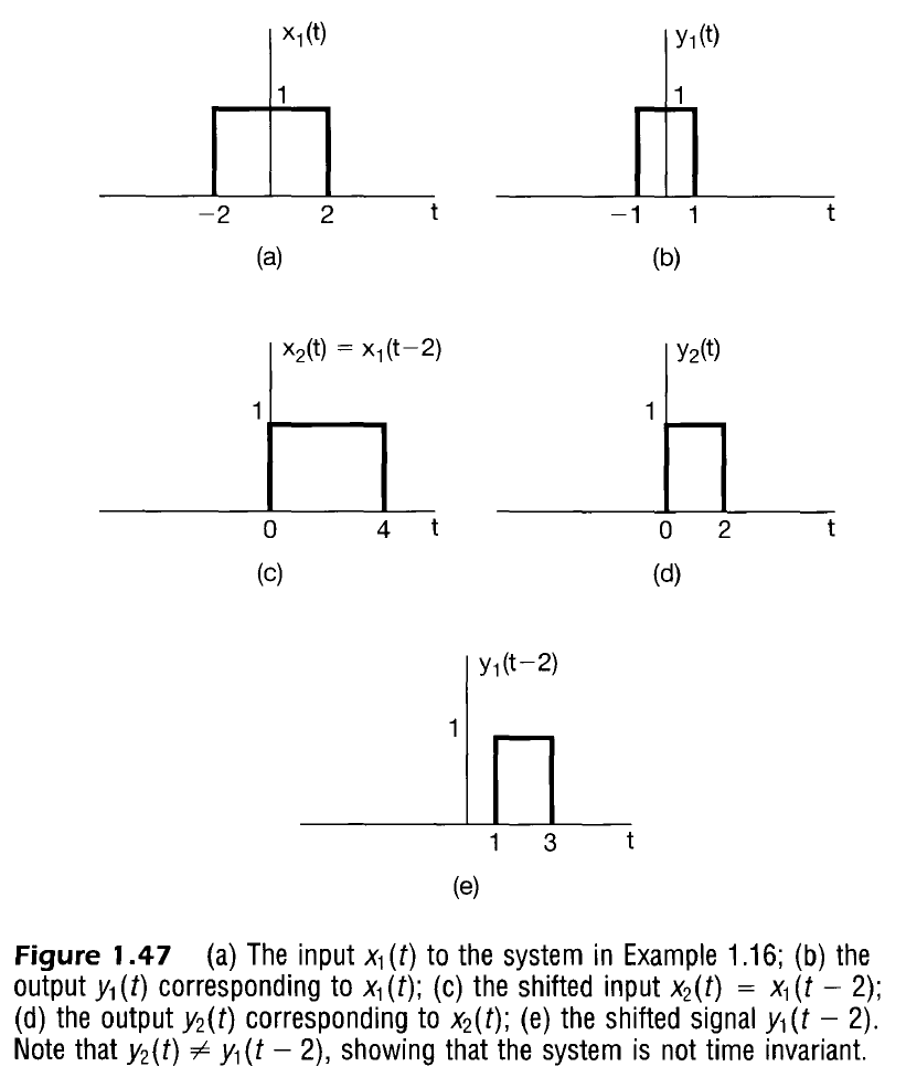
Consider the input signal $x_1(t)$ above. When fed through the system it generates $y_1(t)$, a version compressed around $t=0$.
A shifted input signal $x_2(t) = x_1(t-t_0)$ will produce $y_2(t)$ when compressed. Note that this does not reflect a time shifted version of $y_1(t)$, so the system is not time invariant.
Convolution and LTI Systems
Imagine an impulse centered at $n=k$ represented by $\delta[n-k]$. Assume the system’s response as this impulse is fed through the system is then represented by
$$
\begin{align}
\delta[n-k] \rightarrow h_k[n] \\
\end{align}
$$
If the system is linear, then scaling the impulse at the input yields a correspondingly scaled version of the output.
$$
\begin{align}
a \delta[n-k] \rightarrow a h_k[n] && \text{Linear System}\\
\end{align}
$$
Now, recall the Sampling Property of signals
$$
x[n] \delta[n – n_0] = x[n_0] \delta[n – n_0]
$$
and the corresponding Sifting Property
\begin{align}
x[n] &= \sum_{k = -\infty}^{\infty} x[k] \delta[n-k] \\
\end{align}
Note that the Sifting Property allows us to represent any signal $x[n]$ as a sum of scaled impulses. If the system is linear, then the superposition property allows us to then determine the output as a sum of scaled $h_k[n]$ at each $n$.
$$
\begin{align}
x[n] = \sum_{k = -\infty}^{\infty} x[k] \delta[n-k] \rightarrow y[n] = \sum_{k=-\infty}^{\infty} x[k] h_k[n] \\
\end{align}
$$
Additionally, if the system is time invariant, then we can also assume h_k[n] does not change with each k. If an impulse centered at time $n=0$, $\delta[n]$, causes a time invariant response, $h[n] = h[n]$, then when the input is shifted and scaled, we would also expect to see an identical shift in the response i.e.
$$
\begin{align}
\delta[n] &\rightarrow h[n] \\
x[0]\delta[n] &\rightarrow x[0]h[n] \\
x[k]\delta[n-k] &\rightarrow x[k]h[n-k] \\
x[n] = \sum_{k = -\infty}^{\infty} x[k] \delta[n-k] &\rightarrow y[n] = \sum_{k=-\infty}^{\infty} x[k] h[n-k] \\
\end{align}
$$
This is called the convolution sum which is also represented as
$$y[n] = x[n] * h[n]$$
Convolution
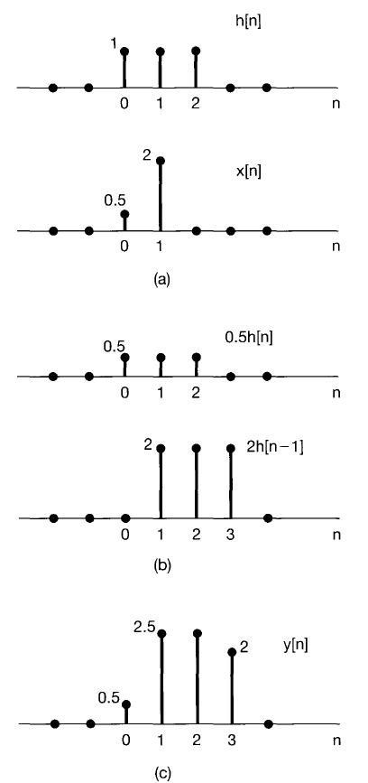
Perspective 1: n-domain
We have generally outlined the n-domain perspective of the convolution sum above, but will rewrite it with visual aids here:
The output of an LTI system with impulse response $h[n]$ at time $n_0$ is a summation of all the $h[n]$’s scaled by each value of $x[n]$ for all time, then the result is evaluated at a specific $n_0$. This perspective can be conceptualized by adding all the scaled $h[n]$’s along the n-axis.
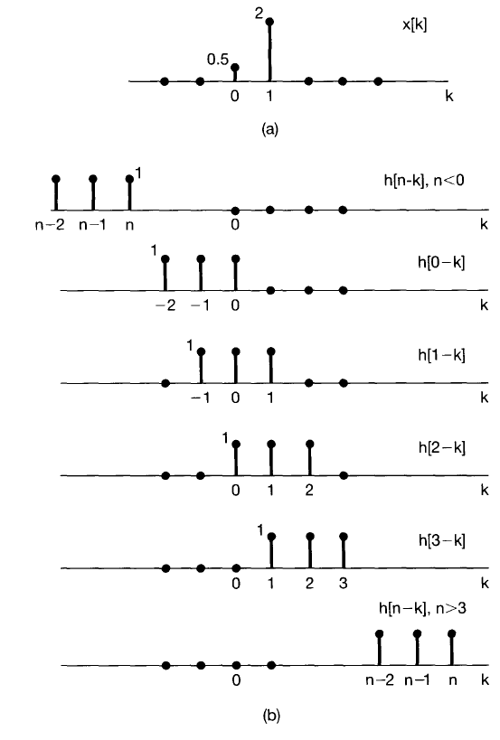
Perspective 2: k-domain
The k-domain perspective can be visualized by imagining the profiles of $x[k]$ and $h[k]$ along the $k$ axis.
$$
y[n] = \sum_{k=-\infty}^{\infty} x[k] h[n-k]
$$
Note that the function $h$ can be interpreted as a shifted and scaled version of itself. $h[n-k]$ can then be conceptualized in one of the following equivalent ways:
- $h[k]$ shifted forward in time by $n$, then flipped about $k=0$ (more ubiquitous shift/scale algorithm, but possibly less intuitive)
- Mirroring $h[k]$ about $k=0$, then delaying the signal by $n$. (Move the $k=0$ position of a flipped $h[k]$ profile ($h[-k]$) to the $k=n$ position).
When $h[n-k]$ is conceptualized in this fashion, the convolution sum is realized using the following steps.
- Fix $x[k]$ in space along the k axis.
- Start with $n=-\infty$ (we will shift the $h[-k]$ all the way to the left at first)
- Flip $h[k]$ at $k=0$, then shift the $h[-k]$ profile from the $k=0$ position to the $k=n$ position.
- At each $k$, multiply the $x$ and $h$ profiles at that spot. The resulting profile is $x[k] h[n-k]$ and note that it is only nonzero in locations that both $x[n]$ and $h[n-k]$ are nonzero.
- Add together all the resulting products (sum profile over all time from $-\infty$ to $\infty$), and that becomes your value for the final $y[n]$
- Increment n by 1 and repeat the process from step 3.
This perspective can also be justified in the following way:
- Assume that when $h[-k]$ is shifted from left to right, the rightmost value of $h[-k]$ overlaps with the leftmost value of $x[k]$ at $k = n_0$. This corresponds to the case when the first scaled impulse of $x[n]$ (using the sifting property) begins creating its scaled input response. The scaled response becomes $y[n]$. Note that if the leftmost nonzero value of $h[k]$ is not at $k=0$, then this result does not get placed at $y[n_0]$.
- At time $n_0 + 1$, the response of $h[-k]$ is again shifted by 1 to the right. This corresponds to the case when the second leftmost value of $x[k]$ begins creating its first scaled input response (it is multiplied by the rightmost value of $h[-k]$. However, the scaled impulse back at the leftmost value of $x[k]$ would be multiplied by the next value of the shifted $h[-k]$ because its nonzero impulse response time has incremented by 1. Both results from the first and second leftmost scaled impulses are added to generate the net result, $y[n + 1]$.
Convolution Properties
Commutative Property
$$
x[n] * h[n] = h[n] * x[n]
$$
Explanation:
$$
\begin{align}
x[n] * h[n] = \sum_{k=-\infty}^{\infty} x[k] h[n – k] \\
\end{align}
$$
Substitute $r = n-k \implies k = n – r$
$$
\begin{align}
x[n] * h[n] &= \sum_{r=\infty}^{-\infty} x[n-r] h[r] \\
x[n] * h[n] &= \sum_{r=-\infty}^{\infty} h[r] x[n-r] \\
x[n] * h[n] &= h[n] * x[n] \\
\end{align}
$$
Distributive Property
$$
\begin{align}
x[n] * (h_1[n] + h_2[n]) = x[n] * h_1[n] + x[n] * h_2[n] \\
(x_1[n] + x_2[n]) * h[n] = x_1[n] * h[n] + x_2[n] * h[n] \\
\end{align}
$$
Associative Property
$$
\begin{align}
x[n] * (h_1[n] * h_2[n]) = (x_1[n] * h_1[n]) * h_2[n]
\end{align}
$$
Impulse Response vs. Step Response
The step response can be directly determined from the impulse response. Assume $s[n]$ is output when $x[n] = u[n]$. From the commutative property
$$
\begin{align}
s[n] &= u[n] * h[n] \\
s[n] &= h[n] * u[n] \\
\end{align}
$$
Note that convolving any signal with $u[n]$ is the same as an accumulator. On the k axis, each value of $h[k]$ before $k=n$ is multiplied by 1 and summed. Therefore, the step response is
$$
\begin{align}
s[n] &= \sum_{k=-\infty}^{n} h[k] \\
\end{align}
$$
Conversely, an impulse can be derived from step signals by
$$
\begin{align}
\delta[n] = u[n] – u[n-1] \\
\end{align}
$$
Therefore, the step response can also be used to determine $h[n]$ if it is unknown.
$$
\begin{align}
\delta[n] * h[n] &= (u[n] – u[n-1]) * h[n] \\
h[n] &= s[n] – s[n-1] \\
\end{align}
$$
This allows us to ultimately characterize any system by the step response.
Other System Properties
Memory
A Memoryless system generates an output signal $y[n]$ from the input signal $x[n]$ and is only dependent on signal information at the same time step, $n$. Some examples of memoryless systems are
$$
\begin{align}
y[n] &= (2x[n] – x^2[n])^2 \\
\end{align}
$$
An examples of a signal with memory is an accumulator
$$
\begin{align}
y[n] &= \sum_{k=-\infty}^n x[k] \\
\end{align}
$$
Invertibility
If a system is invertible, there exists an inverse system such that when the original system is cascaded with the inverse system, the output is the same as the input. In other words, a system is invertible if distinct inputs lead to distinct outputs, and there is a one-to-one correspondence.
If LTI system has impulse response $h[n]$,
$$
\begin{align}
\exists h_i[n] : h[n] * h_i[n] = \delta[n] \implies h[n] \text{ is invertible} \\
\end{align}
$$
Ex: Scaled output
$$
\begin{align}
y(t) &= 2 x(t) \\
h[n] &= 2 \\
h_i[n] &= \frac{1}{2} \\
\end{align}
$$
Ex: Accumulator
$$
\begin{align}
y[n] &= \sum_{k=-\infty}^n x[k] \\
h[n] = u[n] \\
h_i[n] = \delta[n] – \delta[n-1] \\
\end{align}
$$
Ex: Time Shift
$$
\begin{align}
y[n] = x[n-n_0] \\
h[n] = \delta[n-n_0] \\
h_i[n] = \delta[n+n_0] \\
\end{align}
$$
Noninvertible Systems – Multiple inputs yield same output
$$
\begin{align}
y[n] = x^2[n]
\end{align}
$$
Causality
Output only depends on present and past inputs. All memoryless systems are causal.
$$
\begin{align}
\forall n < 0, h[n] = 0 \\
\end{align}
$$
Stability
Suppose input is bounded such that $|x(t)| < B_x$.
$$
\begin{align}
\forall n \in \mathbb{Z}, |x| < B_x, \exists B_y : |y[n]| < B_y \implies \text{ System is Stable}
\end{align}
$$
In general, a system is unstable if small inputs yield diverging response.
If the system is LTI, we may further describe stability:
$$
\begin{align}
|y(t)| &= \left| \int_{-\infty}^{\infty} x(\tau) h(t-\tau) d\tau \right| \\
|y(t)| &= \left| \int_{-\infty}^{\infty} h(\tau) x(t-\tau) d\tau \right| \\
|y(t)| &= \int_{-\infty}^{\infty} |h(\tau)| |x(t-\tau)| d\tau \\
\end{align}
$$
A bounded input suggests
$$
\begin{align}
&|y(t)| \leq |B_x| \int_{-\infty}^{\infty} |h(\tau)| d\tau \\
\\
&\int_{-\infty}^{\infty} |h(\tau)| d\tau < B_y \implies \\
&\text{ System is “Absolutely Integrable”} \implies \\
&\text{ System is Stable} \\
\end{align}
$$
Ex: Pendulum vs. inverted pendulum