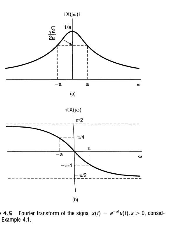
Exponential Decay
$$
\begin{align}
x(t) &= e^{-at} u(t) \\
\\
X(s) &= \int_{-\infty}^{\infty} e^{-at} u(t) e^{-s t} dt \\
X(s) &= \int_{0}^{\infty} e^{-at} e^{-s t} dt \\
X(s) &= \int_{0}^{\infty} e^{-(a + s) t} dt \\
X(s) &= \left[ \frac{1}{-(a + s)} e^{-(a + s) t} \right]_{t=0}^{\infty} \\
X(s) &= \frac{1}{a + s} &Re\{a + s\} > 0\\
X(s) &= \frac{1}{a + s} &Re\{s\} > -Re\{a\}\\
\end{align}
$$
Note that in the Fourier Transform where $s = j\omega$
$$
\begin{align}
|X(j \omega)| = \frac{1}{\sqrt{a^2 + \omega^2}} \\
\\
\angle X(j \omega) = \angle 1 – \angle a + j \omega \\
\angle X(j \omega) = – \text{atan}(\omega/a) \\
\end{align}
$$
Linearity
$$
\begin{align}
x_1(t) &\stackrel{\mathscr{L}}{\leftrightarrow} X_1(s) &&ROC: s \in R_1 \\
x_2(t) &\stackrel{\mathscr{L}}{\leftrightarrow} X_2(s) &&ROC: s \in R_2 \\
\\
a x_1(t) + b x_2(t) &\stackrel{\mathscr{L}}{\leftrightarrow} a X_1(s) + b X_2(s) &&ROC: (s \in R) \land (R_1 \cap R_2 \in R) \\
\end{align}
$$
Note that ROC contains $R_1 \cap R_2$ but may also include additional values outside of $R_1 \cap R_2$. Example of this shown below. Define $x_1$ as
$$
\begin{align}
x_1(t) &= e^{-t} u(t) \\
X_1(s) &= \frac{1}{s + 1} \\
ROC&: Re\{s\} > -1 \\
\end{align}
$$
Then define $x_2$ as
$$
\begin{align}
x_2(t) &= [e^{-t} – e^{-2t}] u(t) \\
X_2(s) &= \int_{-\infty}^{\infty} x_2(t) e^{-st} dt \\
X_2(s) &= \int_{-\infty}^{\infty} [e^{-t} – e^{-2t}] u(t) e^{-st} dt \\
X_2(s) &= \int_{0}^{\infty} [e^{-t} – e^{-2t}] e^{-st} dt \\
X_2(s) &= \int_{0}^{\infty} e^{-t} e^{-st} dt – \int_{0}^{\infty} e^{-2t} e^{-st} dt \\
X_2(s) &= \mathscr{L}\left\{ e^{-t} u(t) \right\} – \mathscr{L}\left\{ e^{-2t} u(t) \right\} &&ROC: (Re\{s\} > -1) \land (Re\{s\} > -2) \\
X_2(s) &= \mathscr{L}\left\{ e^{-t} u(t) \right\} – \mathscr{L}\left\{ e^{-2t} u(t) \right\} &&ROC: Re\{s\} > -1 \\
X_2(s) &= \frac{1}{s+1} – \frac{1}{s+2} &&ROC: Re\{s\} > -1 \\
X_2(s) &= \frac{(s+2)-(s+1)}{(s+1)(s+2)} &&ROC: Re\{s\} > -1 \\
X_2(s) &= \frac{1}{(s+1)(s+2)} &&ROC: Re\{s\} > -1 \\
\end{align}
$$
Note the ROC when we define $x_3$ as
$$
\begin{align}
x_3(t) &= x_1(t) – x_2(t) \\
x_3(t) &= e^{-t} u(t) – [e^{-t} – e^{-2t}] u(t) \\
x_3(t) &= e^{-2t} u(t) \\
X_3(t) &= \frac{1}{s+2} &&ROC: Re\{s\} > -2 \\
\end{align}
$$
ROC for both constituent signals was restrictive, however ROC was modified as we were able to cancel a pole and expand the ROC.
Time Shift
From Synthesis Equation
$$
\begin{align}
x(t) &= \frac{1}{2 \pi} \int_{-\infty}^{\infty} X(s) e^{s t} d\omega \\
x(t-t_0) &= \frac{1}{2 \pi} \int_{-\infty}^{\infty} X(s) e^{s (t-t_0)} d\omega \\
x(t-t_0) &= \frac{1}{2 \pi} \int_{-\infty}^{\infty} X(s) e^{s t} e^{-s t_0} d\omega \\
x(t-t_0) &= \frac{1}{2 \pi} \int_{-\infty}^{\infty} \left[e^{-s t_0} X(s)\right] e^{s t} d\omega \\
\end{align}
$$
In other words, a time delay of $t_0$ is equivalent to multiplying the non-delayed transform by $e^{-st_0}$.
$$
\begin{align}
x(t) &\stackrel{\mathscr{L}}{\leftrightarrow} X(s) \\
x(t-t_0) &\stackrel{\mathscr{L}}{\leftrightarrow} e^{-st_0} X(s) \\
\end{align}
$$
Note that for any finite $t_0$ and $s$, then $e^{-st_0}$ cannot be a pole and the ROC remains unchanged.
s-Domain Shift
This property can be conceptualized as shifting the surface plot of $X(s)$ defined over the entire $s$ plane by $s_0$. On the shifted surface, $X(s-s_0)$, when $s=s_0$ we get the same result that would have previously been at the origin, $X(0)$.
$$
\begin{align}
X(s) &= \int_{-\infty}^{\infty} x(t) e^{-st} dt &&ROC: Re\{s\} \in R \\
\\
X(s-s_0) &= \int_{-\infty}^{\infty} x(t) e^{-(s-s_0)t} dt &&ROC: Re\{s-s_0\} \in R \\
X(s-s_0) &= \int_{-\infty}^{\infty} \left[ x(t) e^{s_0 t} \right] e^{-st} dt &&ROC: Re\{s\} \in R + Re\{s_0\} \\
\\
e^{s_0 t} x(t) &\stackrel{\mathscr{L}}{\leftrightarrow} X(s-s_0) &&ROC: Re\{s\} \in R + Re\{s_0\} \\
\end{align}
$$
In the special case where $s_0 = j \omega_0$ and $x(t)$ is modulated by a sinusoidal signal of frequency $\omega_0$, then we have
$$
\begin{align}
e^{j \omega_0 t} x(t) &\stackrel{\mathscr{L}}{\leftrightarrow} X(s-j \omega_0) &&ROC: Re\{s\} \in R \\
\end{align}
$$
Convolution Property
Recall that the intent of using transforms is to more simply conceptualize the result of convolution in the time domain. The convolution property fully realizes this result.
Laplace Transform
$$
\begin{align}
y(t) &= h(t) * x(t) \\
y(t) &= \int_{-\infty}^{\infty} x(\tau) h(t – \tau) d\tau \\
\\
Y(s) &= \int_{-\infty}^{\infty} \left[ \int_{-\infty}^{\infty} x(\tau) h(t – \tau) d\tau \right] e^{-st} dt \\
Y(s) &= \int_{-\infty}^{\infty} \int_{-\infty}^{\infty} x(\tau) h(t – \tau) e^{-st} d\tau dt \\
Y(s) &= \int_{-\infty}^{\infty} \int_{-\infty}^{\infty} x(\tau) h(t – \tau) e^{-st} dt d\tau \\
Y(s) &= \int_{-\infty}^{\infty} x(\tau) \left[ \int_{-\infty}^{\infty} h(t – \tau) e^{-st} dt \right] d\tau \\
\end{align}
$$
The inner integral may be conceptualized as the transform of a signal $h(t)$ that is time shifted by some value $\tau$. Using the time shift property we then have
$$
\begin{align}
Y(s) &= \int_{-\infty}^{\infty} x(\tau) \left[ H(s) e^{-s\tau} \right] d\tau \\
Y(s) &= H(s) \int_{-\infty}^{\infty} x(\tau) e^{-s\tau} d\tau \\
Y(s) &= H(s) X(s) \\
\end{align}
$$
The two responses $H$ and $X$ just scale each other. The ROC is inclusive of the previous ROC as we saw in the linearity example.
$$
ROC: R_H \cap R_X \in s
$$
Differentiation in Time Domain
Synthesis Equation Approach
$$
\begin{align}
x(t) &\stackrel{\mathscr{L}}{\leftrightarrow} X(s) \\
\\
x(t) &= \frac{1}{2\pi} \int_{-\infty}^{\infty} X(\sigma+j\omega) e^{(\sigma+j\omega)t} d\omega \\
\\
\frac{d}{dt} x(t) &= \frac{d}{dt} \left[ \frac{1}{2\pi} \int_{-\infty}^{\infty} X(\sigma+j\omega) e^{(\sigma+j\omega)t} d\omega \right] \\
\frac{d}{dt} x(t) &= \frac{1}{2\pi} \int_{-\infty}^{\infty} X(\sigma+j\omega) \frac{d}{dt} \left[ e^{(\sigma+j\omega)t} \right] d\omega \\
\frac{d}{dt} x(t) &= \frac{1}{2\pi} \int_{-\infty}^{\infty} X(\sigma+j\omega) \left[ (\sigma+j\omega) e^{(\sigma+j\omega)t} \right] d\omega \\
\frac{d}{dt} x(t) &= \frac{1}{2\pi} \int_{-\infty}^{\infty} \left[ (\sigma+j\omega) X(\sigma+j\omega) \right] e^{(\sigma+j\omega)t} d\omega \\
\\
\frac{d}{dt} x(t) &\stackrel{\mathscr{L}}{\leftrightarrow} (\sigma+j\omega) X(\sigma+j\omega) \\
\frac{d}{dt} x(t) &\stackrel{\mathscr{L}}{\leftrightarrow} s X(s) \\
\\
ROC\left[ X(s) \right]: &s \in R \\
ROC\left[ s X(s) \right]: &s \in R’, R \in R’ \\
\end{align}
$$
Similar to examples above, the ROC for $sX(s)$ may get larger if the added $s$ cancels a pole in $X(s)$ at $s=0$
Bounded Signal Differentiation, Analysis Equation Approach
Reference: https://www.tutorialspoint.com/time-differentiation-property-of-laplace-transform
We sometimes want to use a relation where the Laplace operation is a definite integral (when $x(t)=0$ when outside some bounds $[a, b]$).
$$
\begin{align}
x(t) &\stackrel{\mathscr{L}}{\leftrightarrow} X_0(s) \\
X_0(s) &= \int_a^b x(t) e^{-st} dt \\
\\
\frac{dx(t)}{dt} &\stackrel{\mathscr{L}}{\leftrightarrow} X_1(s) \\
X_1(s) &= \int_a^b \left[ \frac{dx(t)}{dt} \right] e^{-st} dt \\
\end{align}
$$
From IBP
$$
\begin{align}
\int_a^b f(t) g'(t) dt &= [f(t) g(t)]_{t=a}^b – \int_a^b f'(t) g(t) dt \\
\\
f(t) &= e^{-st} \\
f'(t) dt &= – s e^{-st} dt \\
\\
g'(t) dt &= \frac{dx(t)}{dt} dt \\
g(t) &= x(t) \\
\\
X_1(s) &= [e^{-st} x(t)]_{t=a}^b – \int_a^b – s x(t) e^{-st} dt \\
X_1(s) &= [e^{-st} x(t)]_{t=a}^b + s \int_a^b x(t) e^{-st} dt \\
X_1(s) &= [e^{-sb} x(b) – e^{-sa} x(a)] + s \int_a^b x(t) e^{-st} dt \\
X_1(s) &= [e^{-sb} x(b) – e^{-sa} x(a)] + s X_0(s) \\
\end{align}
$$
Initial and Final Value Theorems, Special Cases of Bounded Signal Differentiation in Time Domain
References:
- Introduction to Linear Time-Invariant Dynamic Systems for Students of Engineering (Hallauer) 2.2
- Introduction to Linear Time-Invariant Dynamic Systems for Students of Engineering (Hallauer) 8.2
- Introduction to Linear Time-Invariant Dynamic Systems for Students of Engineering (Hallauer) 8.6
If $\forall t < 0, x(t) = 0$ ($x(t)$ is causal) then we can analyze the special case of the differentiation property where the lower bound is the limit to 0, and the right bound is infinity. This approach allows the use of the impulse function or other discontinuity at $t=0$ in the signal.
$$
\begin{align}
a &= 0^- + 0j = 0^-\\
Re\{b\} &= \infty \\
\\
X_1(s) &= [e^{-s\infty} x(\infty) – e^{-s0^-} x(0^-)] + s X_0(s) \\
X_1(s) &= [0 – 1 \cdot x(0^-)] + s X_0(s) &&\lim_{t \to \infty} e^{-st} x(t) = 0 &\forall t < 0, x(t) = 0 \\
X_1(s) &= s X_0(s) – x(0^-) &&\lim_{t \to \infty} e^{-st} x(t) = 0 &\forall t < 0, x(t) = 0 \\
\end{align}
$$
Note that we assume $e^{-st} x(t)$ converges to 0. If $x(t)$ is of the form $e^{-at}$ then we have the restriction that
$$
\begin{align}
Re\{s\} + Re\{a\} &> 0 \\
Re\{s\} &> – Re\{a\} \\
\end{align}
$$
Substituting $X_1(s)$ in the above equation for the Analysis Equation we can determine the initial value of $x(t)$
$$
\begin{align}
\int_{0^-}^{\infty} \frac{dx(t)}{dt} e^{-st} dt &= s X_0(s) – x(0^-) &&\lim_{t \to \infty} e^{-st} x(t) = 0 &\forall t < 0, x(t) = 0 \\
\int_{0^-}^{0^+} \frac{dx(t)}{dt} e^{-st} dt + \int_{0^+}^{\infty} \frac{dx(t)}{dt} e^{-st} dt &= s X_0(s) – x(0^-) &&\lim_{t \to \infty} e^{-st} x(t) = 0 &\forall t < 0, x(t) = 0 \\
\int_{0^-}^{0^+} \frac{dx(t)}{dt} e^{0} dt + \int_{0^+}^{\infty} \frac{dx(t)}{dt} e^{-st} dt &= s X_0(s) – x(0^-) &&\lim_{t \to \infty} e^{-st} x(t) = 0 &\forall t < 0, x(t) = 0 \\
\int_{0^-}^{0^+} \frac{dx(t)}{dt} dt + \int_{0^+}^{\infty} \frac{dx(t)}{dt} e^{-st} dt &= s X_0(s) – x(0^-) &&\lim_{t \to \infty} e^{-st} x(t) = 0 &\forall t < 0, x(t) = 0 \\
[x(0^+) – x(0^-)] + \int_{0^+}^{\infty} \frac{dx(t)}{dt} e^{-st} dt &= s X_0(s) – x(0^-) &&\lim_{t \to \infty} e^{-st} x(t) = 0 &\forall t < 0, x(t) = 0 \\
x(0^+) + \int_{0^+}^{\infty} \frac{dx(t)}{dt} e^{-st} dt &= s X_0(s) &&\lim_{t \to \infty} e^{-st} x(t) = 0 &\forall t < 0, x(t) = 0 \\
\end{align}
$$
Now if we take the limit as $s \to \infty$ recall we are only considering positive values of $t$, so the value inside the integral becomes 0 for all t (regardless of t). Then we have
$$
\begin{align}
\lim_{s \to \infty} \left[ x(0^+) + \int_{0^+}^{\infty} \frac{dx(t)}{dt} e^{-st} dt \right] &= \lim_{s \to \infty} \left[s X_0(s) \right] &&\lim_{t \to \infty} e^{-st} x(t) = 0 &\forall t < 0, x(t) = 0 \\
x(0^+) + \lim_{s \to \infty} \left[ \int_{0^+}^{\infty} \frac{dx(t)}{dt} e^{-st} dt \right] &= \lim_{s \to \infty} \left[s X_0(s) \right] &&\lim_{t \to \infty} e^{-st} x(t) = 0 &\forall t < 0, x(t) = 0 \\
x(0^+) + \int_{0^+}^{\infty} \frac{dx(t)}{dt} e^{-\infty t} dt &= \lim_{s \to \infty} \left[s X_0(s) \right] &&\lim_{t \to \infty} e^{-st} x(t) = 0 &\forall t < 0, x(t) = 0 \\
x(0^+) &= \lim_{s \to \infty} \left[s X_0(s) \right] &&\lim_{t \to \infty} e^{-st} x(t) = 0 &\forall t < 0, x(t) = 0 \\
\end{align}
$$
Therefore, the initial value of $x(t)$ can be found from $X(s)$. Note that a similar approach may be used if $x(t)$ contains discontinuities elsewhere (for example at another signal boundary).
Note that this property also suggests the order of the numerator of $X(s)$ has to be less than the order of the denominator, otherwise the limit does not converge to a finite value i.e. there is no determinable initial value to the system. Example:
$$
\begin{align}
x(t) = e^{-3 t} u(t) &\stackrel{\mathscr{L}}{\leftrightarrow} X(s) = \frac{1}{s + 3} &&ROC: Re\{s\} > -3 \\
\\
\lim_{Re\{s\} \to \infty} s X(s) &= \lim_{Re\{s\} \to \infty} s \frac{1}{s + 3} \\
\lim_{Re\{s\} \to \infty} s X(s) &= \lim_{Re\{s\} \to \infty} \frac{1}{1 + 3/s} \\
\lim_{Re\{s\} \to \infty} s X(s) &= 1 \\
\end{align}
$$
which matches the expression for $x(t)$ which is known in this case.
Similar analysis can be applied for finding final value
$$
\begin{align}
\lim_{s \to 0} \left[ x(0^+) + \int_{0^+}^{\infty} \frac{dx(t)}{dt} e^{-st} dt \right] &= \lim_{s \to 0} \left[s X_0(s) \right] &&\lim_{t \to \infty} e^{-st} x(t) = 0 &\forall t < 0, x(t) = 0 \\
x(0^+) + \lim_{s \to 0} \left[ \int_{0^+}^{\infty} \frac{dx(t)}{dt} e^{-st} dt \right] &= \lim_{s \to 0} \left[s X_0(s) \right] &&\lim_{t \to \infty} e^{-st} x(t) = 0 &\forall t < 0, x(t) = 0 \\
x(0^+) + \int_{0^+}^{\infty} \frac{dx(t)}{dt} dt &= \lim_{s \to 0} \left[s X_0(s) \right] &&\lim_{t \to \infty} e^{-st} x(t) = 0 &\forall t < 0, x(t) = 0 \\
x(0^+) + [x(\infty) – x(0^+)] &= \lim_{s \to 0} \left[s X_0(s) \right] &&\lim_{t \to \infty} e^{-st} x(t) = 0 &\forall t < 0, x(t) = 0 \\
x(\infty) &= \lim_{s \to 0} \left[s X_0(s) \right] &&\lim_{t \to \infty} e^{-st} x(t) = 0 &\forall t < 0, x(t) = 0 \\
\end{align}
$$
Successive Differentiation
Recall from above (simplified)
$$
\begin{align}
X_0(s) &= \int_a^b x(t) e^{-st} dt \\
X_1(s) &= \int_a^b \left[ \frac{dx(t)}{dt} \right] e^{-st} dt \\
\\
\int_a^b f(t) g'(t) dt &= [f(t) g(t)]_{t=a}^b – \int_a^b f'(t) g(t) dt \\
f(t) &= e^{-st} \\
f'(t) dt &= – s e^{-st} dt \\
g'(t) dt &= \frac{dx(t)}{dt} dt \\
g(t) &= x(t) \\
\\
X_1(s) &= [e^{-st} x(t)]_{t=a}^b – \int_a^b – s x(t) e^{-st} dt \\
X_1(s) &= [e^{-st} x(t)]_{t=a}^b + s \int_a^b x(t) e^{-st} dt \\
X_1(s) &= [e^{-st} x(t)]_{t=a}^b + s X_0(s) \\
\end{align}
$$
Moving on to the next derivative
$$
\begin{align}
X_2(s) &= \int_a^b \frac{d^2 x(t)}{dt^2} e^{-st} dt \\
\\
\int_a^b f(t) g'(t) dt &= [f(t) g(t)]_{t=a}^b – \int_a^b f'(t) g(t) dt \\
f(t) &= e^{-st} \\
f'(t) dt &= – s e^{-st} dt \\
g'(t) dt &= \frac{d^2 x(t)}{dt^2} dt \\
g(t) &= \frac{dx(t)}{dt} \\
\\
X_2(s) &= \left[ e^{-st} \frac{dx(t)}{dt} \right]_{t=a}^b – \int_a^b – s \frac{dx(t)}{dt} e^{-st} dt \\
X_2(s) &= \left[ e^{-st} \frac{dx(t)}{dt} \right]_{t=a}^b + s \int_a^b \frac{dx(t)}{dt} e^{-st} dt \\
X_2(s) &= \left[ e^{-st} x'(t) \right]_{t=a}^b + s X_1(s) \\
X_2(s) &= \left[ e^{-st} x'(t) \right]_{t=a}^b + s \left[ [e^{-st} x(t)]_{t=a}^b + s X_0(s) \right] \\
X_2(s) &= [e^{-st} x'(t)]_{t=a}^b + s[e^{-st} x(t)]_{t=a}^b + s^2 X_0(s) \\
\end{align}
$$
Continuing the trend, we have
$$
\begin{align}
X_n(s) &= [e^{-st} x^{(n-1)}(t)]_{t=a}^b + s[e^{-st} x^{(n-2)}(t)]_{t=a}^b + s^2[e^{-st} x^{(n-3)}(t)]_{t=a}^b + \dots + s^{n-2}[e^{-st} x'(t)]_{t=a}^b + s^{n-1}[e^{-st} x(t)]_{t=a}^b + s^n X_0(s) \\
X_n(s) &= s^n X_0(s) + \sum_{i=0}^{n-1} s^i [e^{-st} x^{(n-1-i)}(t)]_{t=a}^b \\
X_n(s) &= s^n X_0(s) + \sum_{i=0}^{n-1} s^i [e^{-sb} x^{(n-1-i)}(b) – e^{-sa} x^{(n-1-i)}(a)] \\
\end{align}
$$
With some additional assumptions that the signal/system is causal, we have the more commonly seen form
$$
\begin{align}
X_n(s) &= s^n X_0(s) + \sum_{i=0}^{n-1} s^i [e^{-s\infty} x^{(n-1-i)}(\infty) – e^{-s0} x^{(n-1-i)}(0)] &&&\forall t < 0, x(t) = 0 \\
X_n(s) &= s^n X_0(s) + \sum_{i=0}^{n-1} s^i [0 – x^{(n-1-i)}(0)] &&\forall i \in \{0, 1, \dots, n-1\}, \lim_{t \to \infty} e^{-st} x^{(n-1-i)}(t) = 0 &\forall t < 0, x(t) = 0 \\
X_n(s) &= s^n X_0(s) – \sum_{i=0}^{n-1} s^i x^{(n-1-i)}(0) &&\forall i \in \{0, 1, \dots, n-1\}, \lim_{t \to \infty} e^{-st} x^{(n-1-i)}(t) = 0 &\forall t < 0, x(t) = 0 \\
\end{align}
$$
That is if
- We have the 0 order system function and
- Initial conditions for $x(t)$ and its first $n-1$ derivatives and
- $\lim_{t \to \infty} e^{-st} x^i(t) = 0$ for all the $i < n$ derivatives
then we can determine the system function for the $n$th derivative. For a second order system, we have
$$
\begin{align}
X_2(s) &= s^2 X_0(s) – \sum_{i=0}^{1} s^i x^{(1-i)}(0) &&\forall i \in \{0, 1\}, \lim_{t \to \infty} e^{-st} x^{(1-i)}(t) = 0 &&&\forall t < 0, x(t) = 0 \\
X_2(s) &= s^2 X_0(s) – s x(0) – x'(0) &&\lim_{t \to \infty} e^{-st} x(t) = 0 &\lim_{t \to \infty} e^{-st} x'(t) = 0 &&\forall t < 0, x(t) = 0 \\
\end{align}
$$
Differentiation in s-Domain
Fourier Transform
$$
\begin{align}
X(j \omega) &= \int_{-\infty}^{\infty} x(t) e^{-j \omega t} dt \\
\\
\frac{d X(j \omega)}{d \omega} &= \int_{-\infty}^{\infty} -j t x(t) e^{-j \omega t} dt \\
\\
\frac{d^2 X(j \omega)}{d \omega^2} &= \int_{-\infty}^{\infty} (-j t)^2 x(t) e^{-j \omega t} dt \\
\end{align}
$$
So we can generalize
$$
\begin{align}
-j t x(t) &\stackrel{F}{\leftrightarrow} \frac{d X(j \omega)}{d \omega} \\
\\
(-j t)^n x(t) &\stackrel{F}{\leftrightarrow} \frac{d^n X(j \omega)}{d \omega^n} \\
t^n x(t) &\stackrel{F}{\leftrightarrow} (-j)^{-n} \frac{d^n X(j \omega)}{d \omega^n} \\
t^n x(t) &\stackrel{F}{\leftrightarrow} \frac{1}{j^n} \frac{d^n X(j \omega)}{d \omega^n} \\
t^n x(t) &\stackrel{F}{\leftrightarrow} \frac{j^n}{j^n j^n} \frac{d^n X(j \omega)}{d \omega^n} \\
t^n x(t) &\stackrel{F}{\leftrightarrow} \frac{j^n}{(j^2)^n} \frac{d^n X(j \omega)}{d \omega^n} \\
t^n x(t) &\stackrel{F}{\leftrightarrow} \frac{j^n}{(-1)^n} \frac{d^n X(j \omega)}{d \omega^n} \\
t^n x(t) &\stackrel{F}{\leftrightarrow} (-j)^n \frac{d^n X(j \omega)}{d \omega^n} \\
\end{align}
$$
Laplace Transform
Analysis Equation Approach
$$
\begin{align}
x(t) &\stackrel{\mathscr{L}}{\leftrightarrow} X(s) \\
\\
X(s) &= \int_{-\infty}^{\infty} x(t) e^{-st} dt &&ROC: s \in R \\
\\
\frac{d}{ds} X(s) &= \frac{d}{ds} \left[ \int_{-\infty}^{\infty} x(t) e^{-st} dt \right] &&ROC: s \in R \\
\frac{d}{ds} X(s) &= \int_{-\infty}^{\infty} x(t) \frac{d}{ds} \left[ e^{-st} \right] dt &&ROC: s \in R \\
\frac{d}{ds} X(s) &= \int_{-\infty}^{\infty} x(t) \left[ -t e^{-st} \right] dt &&ROC: s \in R \\
\frac{d}{ds} X(s) &= \int_{-\infty}^{\infty} \left[ -t x(t) \right] e^{-st} dt &&ROC: s \in R \\
\\
-t x(t) &\stackrel{\mathscr{L}}{\leftrightarrow} \frac{d}{ds} X(s) &&ROC: s \in R \\
\end{align}
$$
Example
$$
\begin{align}
x(t) &= t e^{-at} u(t) \\
\\
e^{-at} u(t) &\stackrel{\mathscr{L}}{\leftrightarrow} \frac{1}{s + a} &&Re\{s\} > -a \\
\\
-t e^{-at} u(t) &\stackrel{\mathscr{L}}{\leftrightarrow} \frac{d}{ds} \left[ \frac{1}{s + a} \right] &&Re\{s\} > -a \\
-t e^{-at} u(t) &\stackrel{\mathscr{L}}{\leftrightarrow} \frac{d}{ds} \left[ (s + a)^{-1} \right] &&Re\{s\} > -a \\
-t e^{-at} u(t) &\stackrel{\mathscr{L}}{\leftrightarrow} -(s + a)^{-2} \cdot 1 &&Re\{s\} > -a \\
-t e^{-at} u(t) &\stackrel{\mathscr{L}}{\leftrightarrow} – \frac{1}{(s + a)^2} &&Re\{s\} > -a \\
\\
t e^{-at} u(t) &\stackrel{\mathscr{L}}{\leftrightarrow} \frac{1}{(s + a)^2} &&Re\{s\} > -a \\
\end{align}
$$
Successive Differentiation
Note that for successive differentiation, we can see a trend
$$
\begin{align}
-t \cdot t e^{-at} u(t) &\stackrel{\mathscr{L}}{\leftrightarrow} \frac{d}{ds} \frac{1}{(s + a)^2} &&Re\{s\} > -a \\
-t \cdot t e^{-at} u(t) &\stackrel{\mathscr{L}}{\leftrightarrow} -2 \frac{1}{(s + a)^3} &&Re\{s\} > -a \\
\frac{t^2}{2} e^{-at} u(t) &\stackrel{\mathscr{L}}{\leftrightarrow} \frac{1}{(s + a)^3} &&Re\{s\} > -a \\
\\
-t \cdot \frac{t^2}{2} e^{-at} u(t) &\stackrel{\mathscr{L}}{\leftrightarrow} \frac{d}{ds} \frac{1}{(s + a)^3} &&Re\{s\} > -a \\
-t \cdot \frac{t^2}{2} e^{-at} u(t) &\stackrel{\mathscr{L}}{\leftrightarrow} -3 \frac{1}{(s + a)^4} &&Re\{s\} > -a \\
\frac{t^3}{3 \cdot 2} e^{-at} u(t) &\stackrel{\mathscr{L}}{\leftrightarrow} \frac{1}{(s + a)^4} &&Re\{s\} > -a \\
\end{align}
$$
which may be summarized as
$$
\begin{align}
\frac{t^{n-1}}{(n-1)!} e^{-at} u(t) &\stackrel{\mathscr{L}}{\leftrightarrow} \frac{1}{(s + a)^n} &&Re\{s\} > -a \\
\end{align}
$$
which is useful for partial fraction expansion.
Periodic Exponential
In this case, it is easiest to start with the (known) Transformed result and work backwards as a proof. In this case, the transform is a weighted impulse.
$$
\begin{align}
X(j \omega) &= 2 \pi \delta(\omega – \omega_0) \\
\\
x(t) &= \frac{1}{2 \pi} \int_{-\infty}^{\infty} \left[ 2 \pi \delta(\omega – \omega_0) \right] e^{j \omega t} d\omega \\
x(t) &= \int_{-\infty}^{\infty} \delta(\omega – \omega_0) e^{j \omega t} d\omega \\
x(t) &= e^{j \omega_0 t} \\
\end{align}
$$
Note that this also implies
$$
\begin{align}
x(t) = e^{j \omega_0 t} &\stackrel{\mathcal{F}}{\leftrightarrow} X(j \omega) = 2 \pi \delta(\omega – \omega_0) \\
x(t) = a_k e^{j \omega_0 t} &\stackrel{\mathcal{F}}{\leftrightarrow} X(j \omega) = 2 \pi a_k \delta(\omega – \omega_0) \\
\end{align}
$$
If we know a periodic signal in its Fourier Series representation i.e. we know it is a sum of harmonic exponentials, then the Fourier Transform is represented as impulses in the frequency spectrum weighted by $2 \pi a_k$. The kth harmonic is an impulse at $k \omega_0$ with height $2 \pi a_k$.
$$
\begin{align}
x(t) &= \sum_{k=-\infty}^{\infty} a_k e^{j k \omega_0 t} \stackrel{\mathcal{F}}{\leftrightarrow} X(j \omega) = \sum_{k=-\infty}^{\infty} 2 \pi a_k \delta(\omega – k \omega_0) \\
\end{align}
$$
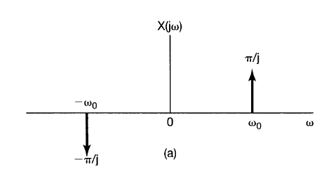
Sin
Fourier Series
$$
\begin{align}
x(t) &= \sin(\omega_0 t) \\
x(t) &= \frac{1}{2 j} \left[ e^{j \omega_0 t} – e^{-j \omega_0 t} \right] \\
\\
a_{1} &= \frac{1}{2j}\\
a_0 &= 0 \\
a_{-1} &= – \frac{1}{2j}\\
\end{align}
$$
Fourier Transform
Recall from the periodic exponential that
$$
\begin{align}
a_k e^{j \omega_0 t} &\stackrel{\mathcal{F}}{\leftrightarrow} 2 \pi a_k \delta(\omega – \omega_0) \\
\end{align}
$$
so if we know the $a_k$s for this signal we can write the Fourier transform as a composition of impulses.
$$
\begin{align}
X(j \omega) &= 2 \pi \left[ – \frac{1}{2j} \right] \delta(\omega + \omega_0) + 2 \pi \left[ \frac{1}{2j} \right] \delta(\omega – \omega_0) \\
X(j \omega) &= – \frac{\pi}{j} \delta(\omega + \omega_0) + \frac{\pi}{j} \delta(\omega – \omega_0) \\
\end{align}
$$
Laplace Transform
$$
\begin{align}
x(t) &= \sin(\omega_0 t) u(t) \\
x(t) &= \frac{1}{2 j} \left[ e^{j \omega_0 t} – e^{-j \omega_0 t} \right] u(t) \\
\end{align}
$$
The Laplace transform of this signal can be represented as
$$
\begin{align}
X(s) &=\frac{1}{2 j} \left[ \mathscr{L}\left\{ e^{j \omega_0 t} u(t) \right\} – \mathscr{L}\left\{ e^{-j \omega_0 t} u(t) \right\} \right] \\
\end{align}
$$
Note that this is essentially a summation of two exponential decay signals, so we can more easily determine the Laplace Transform with some minor manipulation.
$$
\begin{align}
X(s) &=\frac{1}{2 j} \left[ \mathscr{L}\left\{ e^{-(-j \omega_0) t} u(t) \right\} – \mathscr{L}\left\{ e^{-(j \omega_0) t} u(t) \right\} \right] \\
X(s) &=\frac{1}{2 j} \left[ \frac{1}{s + (-j \omega_0)} – \frac{1}{s + (j \omega_0)} \right] &&Re\{s\} > -Re\{-j\omega_0\} \land Re\{s\} > -Re\{j\omega_0\} \\
X(s) &=\frac{1}{2 j} \left[ \frac{1}{s – j \omega_0} – \frac{1}{s + j \omega_0} \right] &&Re\{s\} > 0 \\
X(s) &=\frac{1}{2 j} \frac{(s + j \omega_0) – (s – j \omega_0)}{(s + j \omega_0) (s – j \omega_0)} &&Re\{s\} > 0 \\
X(s) &=\frac{1}{2 j} \frac{2 j \omega_0}{s^2 – (j \omega_0)^2} &&Re\{s\} > 0 \\
X(s) &= \frac{\omega_0}{s^2 + \omega_0^2} &&Re\{s\} > 0 \\
\end{align}
$$
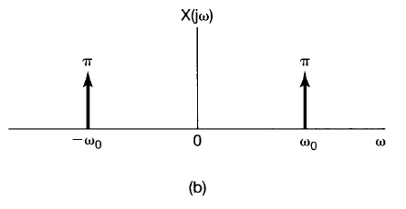
Cos
Fourier Series
Solved similarly to the sin signal above, we have
$$
\begin{align}
x(t) &= \cos(\omega_0 t) \\
x(t) &= \frac{1}{2} \left[ e^{j \omega_0 t} + e^{-j \omega_0 t} \right] \\
\\
a_{1} &= \frac{1}{2}\\
a_0 &= 0 \\
a_{-1} &= – \frac{1}{2}\\
\\
X(j \omega) &= 2 \pi \left[ \frac{1}{2} \right] \delta(\omega + \omega_0) + 2 \pi \left[ \frac{1}{2} \right] \delta(\omega – \omega_0) \\
X(j \omega) &= \pi \delta(\omega + \omega_0) + \pi \delta(\omega – \omega_0) \\
\end{align}
$$
Laplace Transform
$$
\begin{align}
x(t) &= \cos(\omega_0 t) u(t) \\
x(t) &= \frac{1}{2} \left[ e^{j \omega_0 t} + e^{-j \omega_0 t} \right] u(t) \\
\end{align}
$$
The Laplace transform of this signal can be represented as
$$
\begin{align}
X(s) &=\frac{1}{2} \left[ \mathscr{L}\left\{ e^{j \omega_0 t} u(t) \right\} + \mathscr{L}\left\{ e^{-j \omega_0 t} u(t) \right\} \right] \\
\end{align}
$$
Note that this is essentially a summation of two exponential decay signals, so we can more easily determine the Laplace Transform with some minor manipulation.
$$
\begin{align}
X(s) &=\frac{1}{2} \left[ \mathscr{L}\left\{ e^{-(-j \omega_0) t} u(t) \right\} + \mathscr{L}\left\{ e^{-(j \omega_0) t} u(t) \right\} \right] \\
X(s) &=\frac{1}{2} \left[ \frac{1}{s + (-j \omega_0)} + \frac{1}{s + (j \omega_0)} \right] &&Re\{s\} > -Re\{-j\omega_0\} \land Re\{s\} > -Re\{j\omega_0\} \\
X(s) &=\frac{1}{2} \left[ \frac{1}{s – j \omega_0} + \frac{1}{s + j \omega_0} \right] &&Re\{s\} > 0 \\
X(s) &=\frac{1}{2} \frac{(s + j \omega_0) + (s – j \omega_0)}{(s + j \omega_0) (s – j \omega_0)} &&Re\{s\} > 0 \\
X(s) &=\frac{1}{2} \frac{2 s}{s^2 – (j \omega_0)^2} &&Re\{s\} > 0 \\
X(s) &= \frac{s}{s^2 + \omega_0^2} &&Re\{s\} > 0 \\
\end{align}
$$
Impulse
$$
\begin{align}
x(t) &= \delta(t) \\
\\
X(s) &= \int_{-\infty}^{\infty} \delta(t) e^{-s t} dt \\
X(s) &= e^{-s (0)} \\
X(s) &= 1 \\
\end{align}
$$
Fourier transform of an impulse has equal contribution at all frequencies.
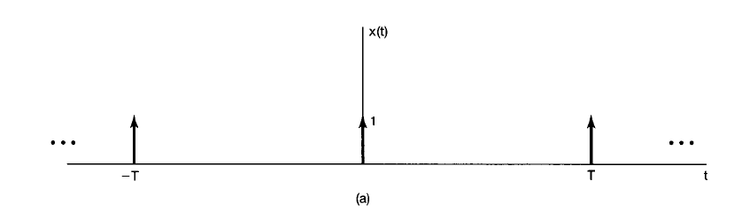
Periodic Impulse Train
$$
\begin{align}
x(t) = \sum_{k=-\infty}^{\infty} \delta(t-kT)
\end{align}
$$
Fourier Series
$$
\begin{align}
a_k &= \frac{1}{T} \int_{-T/2}^{T/2} \delta(t) e^{-j k \omega_0 t} dt \\
a_k &= \frac{1}{T} \int_{-T/2}^{T/2} \delta(0) e^{-j k \omega_0 (0)} dt \\
a_k &= \frac{1}{T} \\
\end{align}
$$
Fourier Transform
We found earlier that if a periodic signal has Fourier Series coefficients $a_k$, then the Fourier Transform may be represented as
$$
\begin{align}
x(t) &= \sum_{k=-\infty}^{\infty} a_k e^{j k \omega_0 t} \stackrel{\mathcal{F}}{\leftrightarrow} X(j \omega) = \sum_{k=-\infty}^{\infty} 2 \pi a_k \delta(\omega – k \omega_0) \\
\end{align}
$$
The Fourier Transform of an impulse train is then
$$
\begin{align}
X(j \omega) = \sum_{k=-\infty}^{\infty} \frac{2 \pi}{T} \delta(\omega – k \omega_0) \\
X(j \omega) = \sum_{k=-\infty}^{\infty} \frac{2 \pi \omega_0}{2 \pi} \delta(\omega – k \omega_0) \\
X(j \omega) = \sum_{k=-\infty}^{\infty} \omega_0 \delta(\omega – k \omega_0) \\
\end{align}
$$
Step
$$
\begin{align}
x(t) &= u(t) \\
x(t) &= \cases{
\begin{array}{ll}
0 &&&t < 0 \\
1 &&&t > 0 \\
\end{array}
} \\
\end{align}
$$
$$
\begin{align}
X(s) &= \int_{-\infty}^{\infty} x(t) e^{-s t} dt \\
X(s) &= \int_{0}^{\infty} 1 \cdot e^{-s t} dt \\
X(s) &= \left[ \frac{1}{-s} e^{-s t} \right]_{t=0}^{\infty} \\
X(s) &= \frac{1}{-s} \left[0-e^{-s (0)} \right] &&Re\{s\} \geq 0 \\
X(s) &= \frac{1}{s} &&Re\{s\} \geq 0 \\
\end{align}
$$
Integration in Time Domain
Fourier Transform
Reference Oppenheim Signals and Systems 4.3.4.
$$
\begin{align}
x(t) &= \frac{1}{2 \pi} \int_{-\infty}^{\infty} X(j \omega) e^{j \omega t} d\omega \\
\int_{-\infty}^t x(\tau) d\tau &= \int_{-\infty}^t \frac{1}{2 \pi} \int_{-\infty}^{\infty} X(j \omega) e^{j \omega \tau} d\omega d\tau \\
\int_{-\infty}^t x(\tau) d\tau &= \frac{1}{2 \pi} \int_{-\infty}^{\infty} X(j \omega) \int_{-\infty}^t e^{j \omega \tau} d\tau d\omega \\
\int_{-\infty}^t x(\tau) d\tau &= \frac{1}{2 \pi} \int_{-\infty}^{\infty} X(j \omega) \left[ \frac{1}{j \omega} e^{j \omega \tau} \right]_{\tau=-\infty}^t d\omega \\
\int_{-\infty}^t x(\tau) d\tau &= \frac{1}{2 \pi} \int_{-\infty}^{\infty} X(j \omega) \left[ \frac{1}{j \omega} e^{j \omega t} \right] d\omega \\
\int_{-\infty}^t x(\tau) d\tau &= \frac{1}{2 \pi} \int_{-\infty}^{\infty} \left[ \frac{1}{j \omega} X(j \omega) \right] e^{j \omega t} d\omega \\
\end{align}
$$
Although it is tempting to jump to the result that
$$
\begin{align}
\int_{-\infty}^t x(\tau) d\tau \stackrel{\mathcal{F}}{\leftrightarrow} \frac{1}{j \omega} X(j \omega) \\
\end{align}
$$
This would neglect evaluation at $\omega = 0$ because $\omega$ exists in the denominator. However, we can further explore the case when $\omega=0$ by referring back to the periodic exponential derivation.
$$
\begin{align}
e^{j \omega_0 t} &\stackrel{\mathcal{F}}{\leftrightarrow} 2 \pi \delta(\omega – \omega_0) \\
1 &\stackrel{\mathcal{F}}{\leftrightarrow} 2 \pi \delta(\omega) \\
\end{align}
$$
As one would expect, the case when $\omega=0$ is essentially the DC or average term. Although it’s not immediately clear how to align this result to the generally accepted result, this forum suggests it is resolved by evaluating the integral by breaking it up into parts.
$$
\begin{align}
\int_{-\infty}^t x(\tau) d\tau &= \frac{1}{2 \pi} \int_{-\infty}^{\infty} X(j \omega) \int_{-\infty}^t e^{j \omega \tau} d\tau d\omega \\
\int_{-\infty}^t x(\tau) d\tau &= \frac{1}{2 \pi} \left[
\int_{-\infty}^{0^-} X(j \omega) \int_{-\infty}^t e^{j \omega \tau} d\tau d\omega +
\int_{C} X(j \omega) \int_{-\infty}^t e^{j \omega \tau} d\tau d\omega +
\int_{0^+}^{\infty} X(j \omega) \int_{-\infty}^t e^{j \omega \tau} d\tau d\omega
\right] \\
\end{align}
$$
The first and third term would be evaluated as we have done above, but the middle term represents the integral as a contour $C$ approaches radius 0 around $\omega=0$. Looking just at this middle term we use a different variable $\theta$ to better describe the contour path.
$$
\begin{align}
\omega &= r e^{j \theta} \\
\frac{d \omega}{d \theta} &= j r e^{j \theta} \\
d \omega &= j r e^{j \theta} d \theta \\
\end{align}
$$
so this term is rewritten
$$
\begin{align}
\int_{C} X(j \omega) \int_{-\infty}^t e^{j \omega \tau} d\tau d\omega &=
\lim_{r \to 0} \int_{-\pi}^0 X(r e^{j \theta}) \int_{-\infty}^t e^{j (r e^{j \theta}) \tau} d\tau \cdot j r e^{j \theta} d \theta \\
\int_{C} X(j \omega) \int_{-\infty}^t e^{j \omega \tau} d\tau d\omega &= \lim_{r \to 0} \int_{-\pi}^0 X(0) j r e^{j \theta} \int_{-\infty}^t e^{j 0 \tau} d\tau d \theta \\
\end{align}
$$
TBD the rest of the analysis. End result is
$$
\begin{align}
\int_{-\infty}^t x(\tau) d\tau \stackrel{\mathcal{F}}{\leftrightarrow} \frac{1}{j \omega} X(j \omega) + \pi X(0) \delta(\omega) \\
\end{align}
$$
I’m not sure if I agree with the last term there as an input signal held as a constant for infinite time does not have finite energy (contradicts parseval’s theorem), so there is limited applicable value there.
Laplace Transform
Direct Approach
$$
\begin{align}
x(t) &= \frac{1}{2 \pi} \int_{-\infty}^{\infty} X(\sigma + j \omega) e^{(\sigma + j \omega) t} d\omega \\
\int_{-\infty}^t x(\tau) d\tau &= \int_{-\infty}^t \frac{1}{2 \pi} \int_{-\infty}^{\infty} X(\sigma + j \omega) e^{(\sigma + j \omega) \tau} d\omega d\tau \\
\int_{-\infty}^t x(\tau) d\tau &= \frac{1}{2 \pi} \int_{-\infty}^{\infty} X(\sigma + j \omega) \int_{-\infty}^t e^{(\sigma + j \omega) \tau} d\tau d\omega \\
\int_{-\infty}^t x(\tau) d\tau &= \frac{1}{2 \pi} \int_{-\infty}^{\infty} X(\sigma + j \omega) \left[ \frac{1}{\sigma + j \omega} e^{(\sigma + j \omega) \tau} \right]_{\tau=-\infty}^t d\omega \\
\int_{-\infty}^t x(\tau) d\tau &= \frac{1}{2 \pi} \int_{-\infty}^{\infty} \frac{1}{\sigma + j \omega} X(s) \left[ e^{(\sigma + j \omega)s \tau} \right]_{\tau=-\infty}^t d\omega \\
\end{align}
$$
Note that if we are to evaluate the quantity in the brackets as the limit approaches negative infinity we have
$$
\begin{align}
\lim_{\tau \to -\infty} e^{(\sigma + j \omega) \tau} &= \lim_{\tau \to -\infty} e^{\sigma \tau} e^{j \omega \tau} \\
\lim_{\tau \to -\infty} e^{(\sigma + j \omega) \tau} &= 0 && \sigma > 0\\
\end{align}
$$
so we have
$$
\begin{align}
\int_{-\infty}^t x(\tau) d\tau &= \frac{1}{2 \pi} \int_{-\infty}^{\infty} \frac{1}{\sigma + j \omega} X(\sigma + j \omega) e^{(\sigma + j \omega) t} d\omega && \sigma > 0 \\
\end{align}
$$
Convolution Approach
We previously found that for the unit step function we have
$$
\begin{align}
u(t) &\stackrel{\mathscr{L}}{\leftrightarrow} \frac{1}{s} &&ROC: Re\{s\} > 0 \\
\end{align}
$$
By noting that integrating a signal in time is essentially convolving the signal with a unit step function, we have
$$
\begin{align}
\int_{-\infty}^{t} x(\tau) d\tau &= x(t) * u(t) \\
\end{align}
$$
Therefore using the convolution property
$$
\begin{align}
x(t) &\stackrel{\mathscr{L}}{\leftrightarrow} X(s) &&ROC: s \in R_X \\
\\
x(t) * u(t) &\stackrel{\mathscr{L}}{\leftrightarrow} \frac{1}{s} X(s) &&ROC: R_X \cap \{ Re\{s\} > 0 \} \in R, s \in R \\
\int_{-\infty}^{t} x(\tau) d\tau &\stackrel{\mathscr{L}}{\leftrightarrow} \frac{1}{s} X(s) &&ROC: R_X \cap \{ Re\{s\} > 0 \} \in R, s \in R \\
\end{align}
$$
Moving Average Example
Reference Exercise 10.2 in Astrom Feedback systems
$$
\begin{align}
\int_{t-a}^t x(\tau) d\tau = \int_{-\infty}^{t} x(\tau) d\tau – \int_{-\infty}^{t-a} x(\tau) d\tau \\
\int_{t-a}^t x(\tau) d\tau = x(t) * u(t) – x(t) * u(t-a) \\
\\
\int_{t-a}^t x(\tau) d\tau \stackrel{\mathscr{L}}{\leftrightarrow} X(s) \frac{1}{s} – X(s) \left[ \frac{1}{s} e^{-sa}\right] \\
\int_{t-a}^t x(\tau) d\tau \stackrel{\mathscr{L}}{\leftrightarrow} \frac{1}{s} X(s) \left[1 – e^{-sa}\right] \\
\end{align}
$$
Time Scaling
$$
\begin{align}
y(t) &= x(at) \\
\\
Y(s) &= \int_{-\infty}^{\infty} y(t) e^{-st} dt \\
Y(s) &= \int_{-\infty}^{\infty} x(at) e^{-st} dt \\
\end{align}
$$
For convenience, define a new variable for integration, $\tau$.
$$
\begin{align}
\tau &= at \\
t &= \frac{\tau}{a} \\
dt &= \frac{1}{a} d\tau \\
\end{align}
$$
The Transform can then be rewritten as
$$
\begin{align}
Y(s) &= \int_{-a\infty}^{a\infty} x(\tau) e^{-(s/a) \tau} \frac{1}{a} d\tau \\
Y(s) &= \frac{1}{a} \int_{-a\infty}^{a\infty} x(\tau) e^{-(s/a) \tau} d\tau \\
\end{align}
$$
$$
Y(s) = \cases{\begin{align}
\frac{1}{a} \int_{-\infty}^{\infty} x(\tau) e^{-(s/a) \tau} d\tau &&a > 0 \\
\frac{1}{a} \int_{\infty}^{-\infty} x(\tau) e^{-(s/a) \tau} d\tau &&a < 0 \\
\end{align}}
$$
$$
Y(s) = \cases{\begin{align}
\frac{1}{a} \int_{-\infty}^{\infty} x(\tau) e^{-(s/a) \tau} d\tau &&a > 0 \\
-\frac{1}{a} \int_{-\infty}^{\infty} x(\tau) e^{-(s/a) \tau} d\tau &&a < 0 \\
\end{align}}
$$
$$
Y(s) = \cases{\begin{align}
\frac{1}{a} X\left(\frac{s}{a}\right) &&a > 0 \\
-\frac{1}{a} X\left(\frac{s}{a}\right) &&a < 0 \\
\end{align}}
$$
$$
Y(s) = \frac{1}{|a|} X\left(\frac{s}{a}\right)
$$
Note that because the output remains bounded (only scaled in magnitude and $s$) ROC can be defined as
$$
\begin{align}
X(s) \rightarrow ROC: s \in R \\
Y(s) \rightarrow ROC: \frac{s}{a} \in R \\
Y(s) \rightarrow ROC: s \in a R \\
\end{align}
$$
Multiplication Property and Frequency Modulation
The synthesis and analysis equations can be written as
$$
\begin{align}
x(t) &= \frac{1}{2 \pi} \int_{-\infty}^{\infty} X(\sigma + j \omega) e^{(\sigma + j \omega) t} d \omega \\
X(\sigma + j \omega) &= \int_{-\infty}^{\infty} x(t) e^{-(\sigma + j \omega) t} dt
\end{align}
$$
Using these two transforms, we can perform the following manipulations
$$
\begin{align}
x_1(t) &\stackrel{\mathscr{L}}{\leftrightarrow} X_1(\sigma + j \omega) \\
x_2(t) &\stackrel{\mathscr{L}}{\leftrightarrow} X_2(\sigma + j \omega) \\
\\
\mathscr{L} \{ x_1(t) x_2(t) \} &= \int_{-\infty}^{\infty} [x_1(t) x_2(t)] e^{-(\sigma + j \omega)t} dt \\
\mathscr{L} \{ x_1(t) x_2(t) \} &= \int_{-\infty}^{\infty} \left[ \frac{1}{2 \pi} \int_{-\infty}^{\infty} X_1(\sigma_1 + j \omega_1) e^{(\sigma_1 + j \omega_1)t} d \omega_1 \right] x_2(t) e^{-(\sigma + j \omega)t} dt \\
\mathscr{L} \{ x_1(t) x_2(t) \} &= \frac{1}{2 \pi} \int_{-\infty}^{\infty} \int_{-\infty}^{\infty} X_1(\sigma_1 + j \omega_1) e^{(\sigma_1 + j \omega_1)t} x_2(t) e^{-(\sigma + j \omega)t} d \omega_1 dt \\
\mathscr{L} \{ x_1(t) x_2(t) \} &= \frac{1}{2 \pi} \int_{-\infty}^{\infty} \int_{-\infty}^{\infty} X_1(\sigma_1 + j \omega_1) x_2(t) e^{-[(\sigma + j \omega) – (\sigma_1 + j \omega_1)]t} d \omega_1 dt \\
\mathscr{L} \{ x_1(t) x_2(t) \} &= \frac{1}{2 \pi} \int_{-\infty}^{\infty} X_1(\sigma_1 + j \omega_1) \left[ \int_{-\infty}^{\infty} x_2(t) e^{-[(\sigma + j \omega) – (\sigma_1 + j \omega_1)]t} dt \right] d \omega_1 \\
\end{align}
$$
Recalling the s-Domain shift property, this can be rewritten as
$$
\begin{align}
\mathscr{L} \{ x_1(t) x_2(t) \} &= \frac{1}{2 \pi} \int_{-\infty}^{\infty} X_1(\sigma_1 + j \omega_1) X_2[(\sigma + j \omega) – (\sigma_1 + j \omega_1)] d \omega_1 \\
\end{align}
$$
In the case where $\sigma = \sigma_1 = 0$ we get the Fourier Transform
$$
\begin{align}
\mathscr{L} \{ x_1(t) x_2(t) \} &= \frac{1}{2 \pi} \int_{-\infty}^{\infty} X_1(j \omega_1) X_2[j (\omega – \omega_1)] d \omega_1 \\
\end{align}
$$
Recognizing the pattern on the RHS, we can see that this is just a convolution between $X_1$ and $X_2$ along the $\omega$ axis or
$$
\begin{align}
x_1(t) x_2(t) \stackrel{\mathscr{L}}{\leftrightarrow} X_1 (\omega) * X_2(j \omega)
\end{align}
$$
Reference: https://www.tutorialspoint.com/time-convolution-and-multiplication-properties-of-laplace-transform
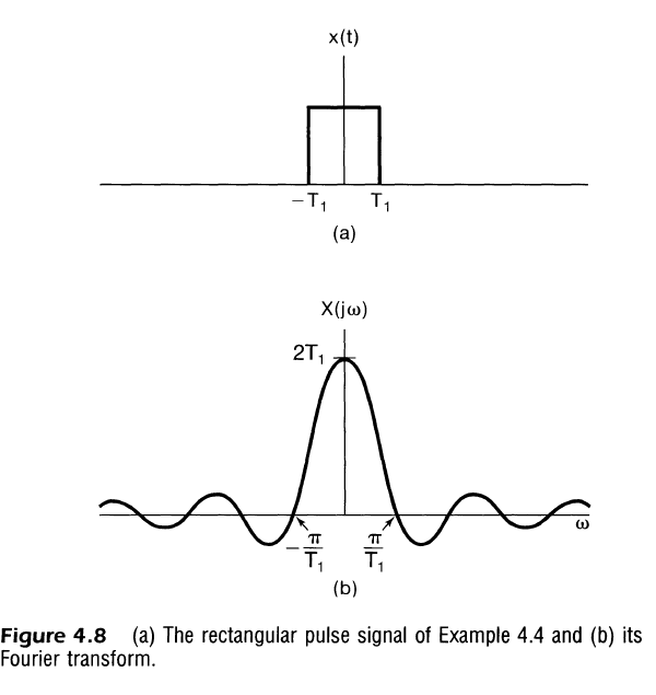
Pulse
$$
\begin{align}
x(t) &= \cases{
\begin{array}{lll}
1 && |t| < T_1 \\
0 && |t| > T_1 \\
\end{array}
} \\
\\
X(s) &= \int_{-\infty}^{\infty} x(t) e^{-s t} dt \\
X(s) &= \int_{-T_1}^{T_1} e^{-s t} dt \\
X(s) &= \left[ \frac{1}{-s} e^{-s t} \right]_{t=-T_1}^{T_1} \\
X(s) &= \frac{1}{-s} \left[ e^{-s T_1} – e^{s T_1}\right] \\
\end{align}
$$
In the case where $Re\{s\} = \sigma = 0$ we get the Fourier Transform
$$
\begin{align}
X(j \omega) &= \frac{1}{-j \omega} \left[ e^{-j \omega T_1} – e^{j \omega T_1}\right] \\
X(j \omega) &= \frac{1}{j \omega} \left[ e^{j \omega T_1} – e^{-j \omega T_1}\right] \\
X(j \omega) &= \frac{1}{j \omega} 2 j \sin(\omega T_1) \\
X(j \omega) &= 2 \frac{\sin(\omega T_1)}{\omega} \\
X(j \omega) &= 2 T_1 \frac{\sin(\omega T_1)}{\omega T_1} \\
X(j \omega) &= 2 T_1 \text{sinc}(\omega T_1) \\
\end{align}
$$
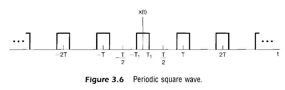
Periodic Pulse/Square Train
Fourier Series
To evaluate one period, it’s generally easiest to look at times $-T/2 < t < T/2$ to define the signal period $T$
$$
x(t) = \cases{
\begin{align}
1 &&&|t| < T_1 \\
0 &&&T_1 < |t| < T/2 \\
\end{align}
}
$$
Plug and Chug Method
$$
\begin{align}
a_0 &= \frac{1}{T} \int_{T} x(t) dt \\
a_0 &= \frac{1}{T} \int_{-T_1}^{T_1} 1 dt \\
a_0 &= \frac{1}{T} 2 T_1 \\
a_0 &= \frac{2 T_1}{T} \\
\end{align}
$$
Note that $a_0$ is the average value of $x(t)$ or duty cycle. For coefficients where $k \neq 0$, we have
$$
\begin{align}
a_k &= \frac{1}{T} \int_{T} x(t) e^{-j k \omega_0 t} dt \\
a_k &= \frac{1}{T} \int_{-T_1}^{T_1} 1 \cdot e^{-j k \omega_0 t} dt \\
a_k &= \frac{1}{T} \left[ \frac{1}{- j k \omega_0} e^{-j k \omega_0 t} \right]_{-T_1}^{T_1} \\
a_k &= – \frac{1}{j k \omega_0 T} \left[ e^{-j k \omega_0 t} \right]_{-T_1}^{T_1} \\
a_k &= – \frac{1}{j k \omega_0 T} \left[ e^{-j k \omega_0 T_1} – e^{j k \omega_0 T_1} \right] \\
a_k &= \frac{1}{j k \omega_0 T} \left[ e^{j k \omega_0 T_1} – e^{-j k \omega_0 T_1} \right] \\
a_k &= \frac{1}{j k \omega_0 T} 2 j \sin(k \omega_0 T_1) \\
a_k &= \frac{2}{T} \frac{\sin(k \omega_0 T_1)}{k \omega_0} \\
a_k &= \frac{2 T_1}{T} \frac{\sin(k \omega_0 T_1)}{k \omega_0 T_1} \\
a_k &= \frac{2 T_1}{T} \text{sinc}(k \omega_0 T_1) \\
\end{align}
$$
Alternatively, it may also be expressed as
$$
\begin{align}
a_k &= a_0 \text{sinc}(k \omega_0 T_1) \\
\end{align}
$$
or
$$
\begin{align}
a_k &= \frac{2}{k (\omega_0 T)} \sin(k \omega_0 T_1) \\
a_k &= \frac{2}{k (2 \pi)} \sin(k \omega_0 T_1) \\
a_k &= \frac{\sin(k \omega_0 T_1)}{k \pi} \\
\end{align}
$$
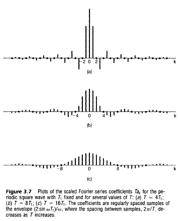
Note that in the case when the duty cycle is 50% (pure square wave), all the nonzero even harmonics are 0, and the 3rd, 5th, and 7th harmonics contain a significant amount of power.
Derivative Property Method
This same result can also be determined using derivatives, time shifts, and takeaways from the impulse train.
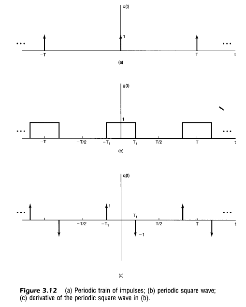
If we define the pulse train as $g(t)$, then
$$
g(t) = \cases{
\begin{align}
1 &&&|t| < T_1 \\
0 &&&T_1 < |t| < T/2 \\
\end{align}
}
$$
and its derivative is
$$
\begin{align}
q(t) &= g'(t) \\
q(t) &= \delta(t + T_1) – \delta(t – T_1) \\
\end{align}
$$
We found earlier that an impulse train has Fourier Series Coefficients represented as
$$
a_k = \frac{1}{T} \\
$$
The composition of the two shifted periodic impulse trains is then
$$
\begin{align}
b_k &= a_k e^{j k \omega_0 T_1} – a_k e^{- j k \omega_0 T_1} \\
b_k &= \frac{1}{T} e^{j k \omega_0 T_1} – \frac{1}{T} e^{- j k \omega_0 T_1} \\
b_k &= \frac{1}{T} [e^{j k \omega_0 T_1} – e^{- j k \omega_0 T_1}] \\
b_k &= \frac{2 j \sin(k \omega_0 T_1)}{T}
\end{align}
$$
The shifted periodic impulse train is the time derivative of the signal, so to now determine the original signal
$$
\begin{align}
c_k &= \frac{b_k}{j k \omega_0} \\
c_k &= \frac{2 j \sin(k \omega_0 T_1)}{j k \omega_0 T} \\
c_k &= \frac{2}{T} \frac{\sin(k \omega_0 T_1)}{k \omega_0} \\
c_k &= \frac{2 T_1}{T} \frac{\sin(k \omega_0 T_1)}{k \omega_0 T_1} \\
c_k &= \frac{2 T_1}{T} \text{sinc}(k \omega_0 T_1) \\
\end{align}
$$
which is the same result as when the coefficients were found directly.
Ideal Lowpass Filter
$$
X(j \omega) = \cases{
\begin{align}
1 && |\omega| < \omega_c \\
0 && |\omega| \geq \omega_c \\
\end{align}
}
$$
$$
\begin{align}
x(t) &= \frac{1}{2 \pi} \int_{-\omega_c}^{\omega_c} 1 \cdot e^{j \omega t} d\omega \\
x(t) &= \frac{1}{2 \pi} \left[ \frac{1}{j t} e^{j \omega t} \right]_{\omega=-\omega_c}^{\omega_c} \\
x(t) &= \frac{1}{j 2 \pi t} \left[ e^{j \omega t} \right]_{\omega=-\omega_c}^{\omega_c} \\
x(t) &= \frac{1}{j 2 \pi t} \left[ e^{j \omega_c t} – e^{-j \omega_c t} \right] \\
x(t) &= \frac{1}{j 2 \pi t} j2 \sin(\omega_c t) \\
x(t) &= \frac{1}{\pi} \frac{\sin(\omega_c t)}{t} \\
x(t) &= \frac{\omega_c}{\pi} \frac{\sin(\omega_c t)}{\omega_c t} \\
x(t) &= \frac{\omega_c}{\pi} \text{sinc}(\omega_c t) \\
\end{align}
$$
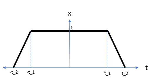
Trapezoidal Signal
To determine the Fourier Transform of a Trapezoidal signal, we use the Time Derivative property in a manner very similar to the Square/Pulse Train.
$$
x(t) = \cases{
\begin{align}
&\frac{t_2 + x}{t_2 – t_1} &&-t_2 \leq t \leq -t_1 \\
&1 &&-t_1 \leq t \leq t_1 \\
&\frac{t_2 – x}{t_2 – t_1} &&t_1 \leq t \leq t_2 \\
&0 && otherwise \\
\end{align}
}
$$
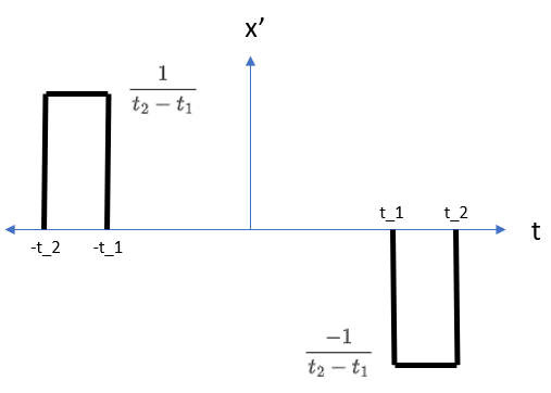
$$
x'(t) = \cases{
\begin{align}
&\frac{1}{t_2 – t_1} &&-t_2 \leq t \leq -t_1 \\
&-\frac{1}{t_2 – t_1} &&t_1 \leq t \leq t_2 \\
&0 && otherwise \\
\end{align}
}
$$
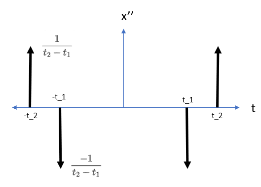
$$
x”(t) =
\frac{1}{t_2 – t_1} \delta(t + t_2) + \frac{-1}{t_2 – t_1} \delta(t + t_1) + \frac{-1}{t_2 – t_1} \delta(t – t_1) + \frac{1}{t_2 – t_1} \delta(t – t_2) \\
$$
Starting from the Fourier Transform of the second derivative
$$
\begin{align}
x”(t) &\stackrel{\mathcal{F}}{\leftrightarrow} X_2(j \omega) \\
\\
X_2(j \omega) &= \frac{1}{t_2 – t_1} 1 \cdot e^{j \omega t_2} + \frac{-1}{t_2 – t_1} 1 \cdot e^{j \omega t_1} + \frac{-1}{t_2 – t_1} 1 \cdot e^{-j \omega t_1} + \frac{1}{t_2 – t_1} 1 \cdot e^{-j \omega t_2} \\
X_2(j \omega) &= \frac{1}{t_2 – t_1} (e^{j \omega t_2} + e^{-j \omega t_2}) – \frac{1}{t_2 – t_1} (e^{j \omega t_1} + e^{-j \omega t_1}) \\
X_2(j \omega) &= \frac{1}{t_2 – t_1} [(e^{j \omega t_2} + e^{-j \omega t_2}) – (e^{jt_1} + e^{-jt_1})] \\
X_2(j \omega) &= \frac{1}{t_2 – t_1} [2\cos(\omega t_2) – 2\cos(\omega t_1)] \\
X_2(j \omega) &= \frac{2}{t_2 – t_1} [\cos(\omega t_2) – \cos(\omega t_1)] \\
\end{align}
$$
We can simplify this notation using the identity
$$
\cos(\theta – \phi) – \cos(\theta + \phi) = 2 \sin(\theta) \sin(\phi)
$$
So let’s define
$$
\begin{align}
t_{rf} &= t_2 – t_1 \\
t_{pw} &= 2(t_1 + t_{rf}/2) \\
\\
\theta &= \omega (t_1 + t_{rf}/2) \\
\theta &= \omega (t_{pw}/2) \\
\\
\phi &= \omega (t_{rf}/2) \\
\\
\theta – \phi &= \omega (t_1 + t_{rf}/2) – \omega (t_{rf}/2) \\
\theta – \phi &= \omega (t_1 + t_{rf}/2 – t_{rf}/2) \\
\theta – \phi &= \omega t_1 \\
\\
\theta + \phi &= \omega (t_1 + t_{rf}/2) + \omega (t_{rf}/2) \\
\theta + \phi &= \omega (t_1 + t_{rf}/2 + t_{rf}/2) \\
\theta + \phi &= \omega (t_1 + t_{rf}) \\
\theta + \phi &= \omega t_2 \\
\end{align}
$$
which gives
$$
\begin{align}
X_2(s) &= \frac{2}{t_{rf}} 2 \sin(\theta) \sin(\phi) \\
X_2(s) &= \frac{4}{t_{rf}} \sin(\theta) \sin(\phi) \\
\\
X_1(s) &= \frac{4}{(j \omega) t_{rf}} \sin(\theta) \sin(\phi) \\
\\
X(s) &= \frac{4}{(j \omega)^2 t_{rf}} \sin(\theta) \sin(\phi) \\
X(s) &= \frac{4}{(j \omega)^2 t_{rf}} \sin(\omega t_{pw}/2) \sin(\omega t_{rf} / 2) \\
X(s) &= \frac{4 (\omega t_{pw}/2) (\omega t_{rf}/2)}{(j \omega)^2 t_{rf}} \frac{\sin(\omega t_{pw}/2)}{(\omega t_{pw}/2)} \frac{\sin(\omega t_{rf} / 2)}{(\omega t_{rf}/2)} \\
X(s) &= \frac{t_{pw}}{-1} \text{sinc}(\omega t_{pw}/2) \text{sinc}(\omega t_{rf} / 2) \\
X(s) &= -t_{pw} \text{sinc}(\omega t_{pw}/2) \text{sinc}(\omega t_{rf} / 2) \\
\end{align}
$$
Power Analysis
The power contained in the frequency spectrum in dB would be
$$
\begin{array}{ll}
P_{dB} = 20 \log_{10}(|X(s)|) \\
P_{dB} = 20 \log_{10}[|-t_{pw} \text{sinc}(\omega t_{pw}/2) \text{sinc}(\omega t_{rf}/2)|] \\
P_{dB} = 20 \log_{10}(|-t_{pw}|) + 20 \log_{10}(|\text{sinc}(\omega t_{pw}/2)|) + 20 \log_{10}(|\text{sinc}(\omega t_{rf}/2)|) \\
P_{dB} = 20 \log_{10}(t_{pw}) + 20 \log_{10}(|\text{sinc}(\omega t_{pw}/2)|) + 20 \log_{10}(|\text{sinc}(\omega t_{rf}/2)|) \\
\end{array}
$$
As mentioned on the page regarding the special sinc function, $\text{sinc}(x)$ may be approximated as a constant value for small magnitudes of $x$ and $1/x$ for larger values. These two curves would meet at $x = 1$.
$$
P_{sinc,dB}(x) \approx \cases{
\begin{array}{ll}
0 &|x| < 1 \\
-20 log_{10}(x) &|x| \geq 1 \\
\end{array}
} \\
$$
Using this principle, we have the curve intersections for the second term occurring at
$$
\begin{align}
\omega_{intersect} t_{pw}/2 = 1 \\
\omega_{intersect} = 2/t_{pw} \\
\end{align}
$$
and for the third term
$$
\begin{align}
\omega_{intersect} t_{rf}/2 = 1 \\
\omega_{intersect} = 2/t_{rf} \\
\end{align}
$$
Assuming $t_{rf} < t_{pw}$, note that $\omega_{intersect, rf} > \omega_{intersect, pw}$ suggesting that the first roll-off frequency is dependent on the pulse width. We now would have the power curve approximately look like
$$
P_{dB} \approx \cases{
\begin{array}{ll}
20 \log_{10}(t_{pw}) &0 < \omega < 2/t_{pw} < 2/t_{rf} \\
20 \log_{10}(t_{pw}) – 20 \log_{10} (\omega t_{pw} / 2) &0 < 2/t_{pw} < \omega < 2/t_{rf} \\
20 \log_{10}(t_{pw}) – 20 \log_{10} (\omega t_{pw} / 2) – 20 \log_{10} (\omega t_{rf} / 2) &0 < 2/t_{pw} < 2/t_{rf} < \omega \\
\end{array}
}
$$
This curve effectively looks like a constant, then a 20 dB/decade drop, then an increase to 40 dB/decade drop depending on the pulse width and the rise/fall time.
Single Ramp
$$
x(t) = \cases{
\begin{align}
&0 &&t < -t_r/2 \\
&\frac{t + t_r/2}{t_r} &&-t_r/2 < t < t_r/2 \\
&1 &&t > t_r/2 \\
\end{align}
}
$$
$$
x'(t) = \cases{
\begin{align}
&\frac{1}{t_r} &&-t_r/2 < t < t_r/2 \\
&0 &&\text{Otherwise} \\
\end{align}
}
$$
$$
\begin{align}
x”(t) &= \frac{1}{t_r} [\delta(t+t_r/2) – \delta(t-t_r/2)] \\
\\
X_2(j \omega) &= \frac{1}{t_r} [e^{j \omega t_r/2} – e^{-j \omega t_r/2}] \\
X_2(j \omega) &= \frac{2 j}{t_r} \sin(\omega t_r/2) \\
\\
X_1(j \omega) &= \frac{2 j}{(j \omega) t_r} \sin(\omega t_r/2) \\
\\
X(j \omega) &= \frac{2 j}{(j \omega)^2 t_r} \sin(\omega t_r/2) \\
X(j \omega) &= \frac{2 j (\omega t_r/2)}{(j \omega)^2 t_r} \frac{\sin(\omega t_r/2)}{(\omega t_r/2)} \\
X(j \omega) &= \frac{1}{j \omega} \text{sinc}(\omega t_r/2) \\
\end{align}
$$
Note that this makes sense because $x(t)$ can also be expressed as
$$
x(t) = u(t) * p(t)
$$
where $u(t)$ is the unit step function and $p(t)$ is a pulse signal.
$$
p(t) = \cases{
\begin{align}
&\frac{1}{t_r} && -t_r/2 < t < t_r/2 \\
&0 &&\text{Otherwise} \\
\end{align}
}
$$
Paying attention to how we substitute the pulse width variables into the pulse equation, we have
$$
\begin{align}
X(j \omega) &= U(j \omega) P(j \omega) \\
X(j \omega) &= \left[ \frac{1}{j \omega} \right] \left[\frac{1}{t_r} 2 (t_r/2) \text{sinc}(\omega (t_r/2)) \right] \\
X(j \omega) &= \frac{1}{j \omega} \text{sinc}(\omega t_r/2) \\
\end{align}
$$
Power Analysis
$$
\begin{align}
|X(j \omega)| &= \left|\frac{1}{j \omega}\right| |\text{sinc}(\omega t_r/2)| \\
|X(j \omega)| &= \frac{1}{\omega} |\text{sinc}(\omega t_r/2)| \\
\\
P_{X,dB} &= 20 \log_{10} (1/\omega) + 20 \log_{10} |\text{sinc}(\omega t_r / 2)| \\
P_{X,dB} &= -20 \log_{10}(\omega) + 20 \log_{10}|\text{sinc}(\omega t_r / 2)| \\
\end{align}
$$
Approximating the power of the sinc function as two stepwise functions
$$
P_{sinc,dB}(x) \approx \cases{
\begin{array}{ll}
0 &|x| < 1 \\
-20 log_{10}(x) &|x| \geq 1 \\
\end{array}
} \\
$$
We have the curve intersection at
$$
\begin{align}
\omega_{intersect} t_r/2 = 1 \\
\omega_{intersect} = 2/t_r \\
\end{align}
$$
So
$$
P_{X,dB} = \cases{
\begin{align}
&-20 \log_{10}(\omega) && \omega < 2/t_r \\
&-20 \log_{10}(\omega) -20\log_{10}(\omega t_r / 2) && \omega > 2/t_r \\
\end{align}
}
$$
Which looks like a decrease of -20 dB/decade until $\omega = 2/t_r$ when it switches to -40 dB/decade.
Triangular Spike
Triangular spike of height 1 and width $t_{pw}$ centered around $t = 0$. See Trapezoidal Signal analysis for reference on steps.
$t_{pw}$ represents the total width of the spike.
$$
x(t) = \cases{
\begin{align}
\frac{2}{t_{pw}}t + 1 &&&-\frac{t_{pw}}{2} < t < 0 \\
\frac{-2}{t_{pw}}t + 1 &&&0 < t < \frac{t_{pw}}{2} \\
0 &&&\text{Otherwise} \\
\end{align}
}
$$
$$
x”(t) = \frac{-4}{t_{pw}} \delta(t) + \frac{2}{t_{pw}} \left[ \delta(t + \frac{t_{pw}}{2}) + \delta(t – \frac{t_{pw}}{2}) \right]
$$
$$
\begin{align}
x(t) &\stackrel{\mathscr{L}}{\leftrightarrow} X(s) \\
x”(t) &\stackrel{\mathscr{L}}{\leftrightarrow} X”(s) \\
\delta(t) &\stackrel{\mathscr{L}}{\leftrightarrow} 1 \\
\end{align}
$$
$$
\begin{align}
X”(j \omega) &= \frac{-4}{t_{pw}} + \frac{2}{t_{pw}} \left[ e^{j \omega t_{pw}/2} + e^{-j \omega t_{pw}/2} \right] \\
X”(j \omega) &= \frac{-4}{t_{pw}} + \frac{2}{t_{pw}} 2 \cos\left(\frac{1}{2} \omega t_{pw}\right) \\
X”(j \omega) &= \frac{4}{t_{pw}} \left[ \cos\left(\frac{1}{2} \omega t_{pw}\right) – 1 \right] \\
\end{align}
$$
Half Angle Formula
$$
\begin{align}
\sin^2(x) &= \frac{1 – \cos(2x)}{2} \\
2 \sin^2(x) &= 1 – \cos(2x) \\
\cos(2x) – 1 &= – 2 \sin^2(x)
\end{align}
$$
$$
\begin{align}
X”(j \omega) &= \frac{4}{t_{pw}} \left[ -2 \sin^2\left(\frac{1}{4} \omega t_{pw}\right) \right] \\
X”(j \omega) &= – \frac{8}{t_{pw}} \sin^2\left(\frac{1}{4} \omega t_{pw}\right) \\
\\
X(j \omega) &= \frac{X”(\omega)}{(j \omega)^2} \\
X(j \omega) &= – \frac{8}{t_{pw}} \frac{\sin^2(\omega t_{pw}/4)}{(j \omega)^2} \\
X(j \omega) &= \frac{8 (t_{pw}/4)^2}{t_{pw}} \frac{\sin^2(\omega t_{pw}/4)}{\omega^2(t_{pw}/4)^2} \\
X(j \omega) &= \frac{8 t_{pw}}{16} \left[ \frac{\sin(\omega t_{pw}/4)}{\omega t_{pw}/4} \right]^2 \\
X(j \omega) &= \frac{t_{pw}}{2} \text{sinc}^2(\omega t_{pw}/4) \\
\end{align}
$$
Power Analysis
Frequency response for sinc function
$$
\begin{align}
P_{dB}(\omega) &= 20 \log_{10} X(j\omega) \\
P_{dB}(\omega) &= 20 \log_{10} \left[ \frac{t_{pw}}{2} \text{sinc}^2(\omega t_{pw}/4) \right] \\
P_{dB}(\omega) &= 20 \log_{10} \left[ \frac{t_{pw}}{2} \right] + 20 \log_{10} \left[ \text{sinc}^2(\omega t_{pw}/4) \right] \\
P_{dB}(\omega) &= 20 \log_{10} \left[ \frac{t_{pw}}{2} \right] + 40 \log_{10} \left[ \text{sinc}(\omega t_{pw}/4) \right] \\
\end{align}
$$
Recall that sinc function on logarithmic graph may be represented as
$$
\log_{10} \text{sinc}(x) \approx \cases{
\begin{align}
&\log_{10}1 = 0 &&x < 1 \\
&\log_{10}\frac{1}{x} = – \log_{10}x &&x > 1 \\
\end{align}
}
$$
Intersection point is
$$
\begin{align}
\frac{\omega t_{pw}}{4} &= 1 \\
\omega &= \frac{4}{t_{pw}} \\
\end{align}
$$
So frequency response may be estimated as
$$
P_{dB}(\omega) \approx
\cases{
\begin{align}
&20 \log_{10} \left[ \frac{t_{pw}}{2} \right] &&\omega < \frac{4}{t_{pw}} \\
&20 \log_{10} \left[ \frac{t_{pw}}{2} \right] – 40 \log_{10} \left[ \frac{\omega t_{pw}}{4} \right] &&\omega > \frac{4}{t_{pw}} \\
\end{align}
}
$$
or in terms of frequency $f = \omega / 2 \pi$
$$
P_{dB}(f) \approx
\cases{
\begin{align}
&20 \log_{10} \left[ \frac{t_{pw}}{2} \right] &&f < \frac{2}{\pi t_{pw}} \\
&20 \log_{10} \left[ \frac{t_{pw}}{2} \right] – 40 \log_{10} \left[ \frac{\pi f t_{pw}}{2} \right] &&f < \frac{2}{\pi t_{pw}} \\
\end{align}
}
$$
Note that as $t_{pw}$ gets smaller, the roll-off frequency moves to higher frequencies.
- For spike 1 ms wide, cutoff frequency is 637 Hz
- For spike 100 us wide, cutoff frequency is 6.37 kHz
Conjugation, Complex Symmetry, Even, and Odd
Consider the signal and transform pair
$$
\begin{align}
x(t) &\stackrel{\mathcal{F}}{\leftrightarrow} X(j \omega) \\
\end{align}
$$
The complex conjugate of the Analysis Equation is then
$$
\begin{align}
X^*(j \omega) &= \left[ \int_{-\infty}^{\infty} x(t) e^{-j \omega t} dt \right]^* \\
\end{align}
$$
Note that the complex conjugate of a product has the following property
$$
\begin{align}
\left[ (\sigma_1 + j \omega_1) (\sigma_2 + j \omega_2) \right]^* &= \left[ \sigma_1 \sigma_2 + j (\sigma_1 \omega_2 + \sigma_2 \omega_1) – \omega_1 \omega_2 \right]* \\
\left[ (\sigma_1 + j \omega_1) (\sigma_2 + j \omega_2) \right]^* &= \left[ (\sigma_1 \sigma_2 – \omega_1 \omega_2) + j (\sigma_1 \omega_2 + \sigma_2 \omega_1) \right]* \\
\left[ (\sigma_1 + j \omega_1) (\sigma_2 + j \omega_2) \right]^* &= (\sigma_1 \sigma_2 – \omega_1 \omega_2) – j (\sigma_1 \omega_2 + \sigma_2 \omega_1) \\
\\
(\sigma_1 + j \omega_1)^* (\sigma_2 + j \omega_2)^* &= (\sigma_1 – j \omega_1) (\sigma_2 – j \omega_2) \\
(\sigma_1 + j \omega_1)^* (\sigma_2 + j \omega_2)^* &= \sigma_1 \sigma_2 – j (\sigma_1 \omega_2 + \sigma_2 \omega_1) – \omega_1 \omega_2 \\
(\sigma_1 + j \omega_1)^* (\sigma_2 + j \omega_2)^* &= (\sigma_1 \sigma_2 -\omega_1 \omega_2) – j (\sigma_1 \omega_2 + \sigma_2 \omega_1) \\
&\implies \\
[ab]^* &= a^* b^* \\
\end{align}
$$
so we can write
$$
\begin{align}
X^*(j \omega) &=\int_{-\infty}^{\infty} \left[ x(t) e^{-j \omega t} \right]^* dt \\
X^*(j \omega) &=\int_{-\infty}^{\infty} x^*(t) e^{j \omega t} dt \\
\end{align}
$$
The following statements are therefore also true.
$$
\begin{align}
X^*(-j \omega) &=\int_{-\infty}^{\infty} x^*(t) e^{-j \omega t} dt \\
\\
x^*(t) &\stackrel{\mathcal{F}}{\leftrightarrow} X^*(-j \omega) \\
\end{align}
$$
A notable corollary of this concerns real signals. A real signal has $x(t) = x^*(t)$ so therefore
$$
\begin{align}
X^*(-j \omega) &=\int_{-\infty}^{\infty} x^*(t) e^{-j \omega t} dt \\
X^*(-j \omega) &=\int_{-\infty}^{\infty} x(t) e^{-j \omega t} dt \\
X^*(-j \omega) &= X(j \omega) \\
X^*(j \omega) &= X(-j \omega) \\
\end{align}
$$
Another finding concerns real even signals where $x(t) = x(-t)$
$$
\begin{align}
X(j \omega) &= \int_{-\infty}^{\infty} x(t) e^{-j \omega t} dt \\
X(-j \omega) &= \int_{-\infty}^{\infty} x(t) e^{j \omega t} dt \\
\\
t = -\tau &\implies \\
X(-j \omega) &= \int_{-\infty}^{\infty} x(-\tau) e^{-j \omega \tau} d\tau \\
X(-j \omega) &= \int_{-\infty}^{\infty} x(\tau) e^{-j \omega \tau} d\tau \\
X(-j \omega) &= X(j \omega) \\
\end{align}
$$
In other words, even signals have even Fourier Transforms.
Similarly for odd functions where $-x(t) = x(-t)$
$$
\begin{align}
X(j \omega) &= \int_{-\infty}^{\infty} x(t) e^{-j \omega t} dt \\
X(-j \omega) &= \int_{-\infty}^{\infty} x(t) e^{j \omega t} dt \\
\\
t = -\tau &\implies \\
X(-j \omega) &= \int_{-\infty}^{\infty} x(-\tau) e^{-j \omega \tau} d\tau \\
X(-j \omega) &= -\int_{-\infty}^{\infty} x(\tau) e^{-j \omega \tau} d\tau \\
X(-j \omega) &= -X(j \omega) \\
\end{align}
$$
Therefore, real odd signals have odd Fourier Transforms.
Parseval’s Theorem
See 4.3.7 in Oppenheim Signals and Systems.
Consider the signal and transform pair
$$
\begin{align}
x(t) &\stackrel{\mathcal{F}}{\leftrightarrow} X(j \omega) \\
\end{align}
$$
The energy in the signal is
$$
\begin{align}
\int_{-\infty}^{\infty} |x(t)|^2 dt &= \int_{-\infty}^{\infty} x(t) x^*(t) dt
\end{align}
$$
From our analysis of complex signals
$$
\begin{align}
x^*(t) &\stackrel{\mathcal{F}}{\leftrightarrow} X^*(-j \omega) \\
\\
\int_{-\infty}^{\infty} |x(t)|^2 dt &= \int_{-\infty}^{\infty} x(t) \left[ \frac{1}{2 \pi} \int_{-\infty}^{\infty} X^*(-j \omega) e^{j \omega} d \omega \right] dt \\
\int_{-\infty}^{\infty} |x(t)|^2 dt &= \int_{-\infty}^{\infty} x(t) \left[ \frac{1}{2 \pi} \int_{-\infty}^{\infty} X^*(j \omega) e^{-j \omega} d \omega \right] dt \\
\int_{-\infty}^{\infty} |x(t)|^2 dt &= \frac{1}{2 \pi} \int_{-\infty}^{\infty} \int_{-\infty}^{\infty} x(t) X^*(j \omega) e^{-j \omega} d \omega dt \\
\int_{-\infty}^{\infty} |x(t)|^2 dt &= \frac{1}{2 \pi} \int_{-\infty}^{\infty} \left[ \int_{-\infty}^{\infty} x(t) e^{-j \omega} dt \right] X^*(j \omega) d \omega \\
\int_{-\infty}^{\infty} |x(t)|^2 dt &= \frac{1}{2 \pi} \int_{-\infty}^{\infty} X(j \omega) X^*(j \omega) d \omega \\
\int_{-\infty}^{\infty} |x(t)|^2 dt &= \frac{1}{2 \pi} \int_{-\infty}^{\infty} |X(j \omega)|^2 d \omega \\
\end{align}
$$
In short the finite energy in a signal is related to the finite energy in the energy density spectrum by a scaling factor, $1/2\pi$.
For a constant signal that hypothetically exists for all time e.g. $x(t)=1 \stackrel{\mathcal{F}}{\leftrightarrow} 2 \pi \delta(\omega)$, the theorem does not directly apply. However, if we consider a constant signal over a finite time period T, then the theorem would hold for that time-limited signal. As T approaches infinity, the energy of the signal also approaches infinity, which aligns with our intuitive understanding of a constant signal existing for all time.