Sampling of Discrete Signals

Taking a sample every $N$ steps of the input signal and setting $N-1$ samples in between to zero

$$
x_p[n] = \cases{
\begin{align}
x[n] && n/N \in \mathbb{Z} \\
0 &&\text{Otherwise}
\end{align}}
$$

$$
\begin{align}
x_p[n] &= x[n] \sum_{k=-\infty}^{\infty} \delta[n – kN] \\
x_p[n] &= \sum_{k=-\infty}^{\infty} x[n] \delta[n – kN] \\
x_p[n] &= \sum_{k=-\infty}^{\infty} x[kN] \delta[n – kN] \\
\end{align}
$$

We can also describe $x_p[n]$ in another form

$$
\begin{align}
x_p[n] &= p[n] x[n] \\
\end{align}
$$

Where

$$
\begin{align}

p[n] = \sum_{k=-\infty}^{\infty} \delta[n – kN] &\stackrel{\mathcal{F}}{\leftrightarrow} P(e^{j \omega}) = \sum_{k=-\infty}^{\infty} \frac{2 \pi}{N} \delta(\omega – k \frac{2 \pi}{N}) \\

p[n] = \sum_{k=-\infty}^{\infty} \delta[n – kN] &\stackrel{\mathcal{F}}{\leftrightarrow} P(e^{j \omega}) = \omega_s \sum_{k=-\infty}^{\infty} \delta(\omega – k \omega_s) \\
\end{align}
$$

Then, using the multiplication property

$$
\begin{align}
X_p(e^{j \omega}) &= \frac{1}{2 \pi} \int_{2 \pi} P(e^{j \theta}) X(e^{j (\omega – \theta)}) d \theta \\

X_p(e^{j \omega}) &= \frac{1}{2 \pi} \int_{2 \pi} \left[ \frac{2 \pi}{N} \sum_{k=-\infty}^{\infty} \delta(\theta – k \frac{2 \pi}{N}) \right] X(e^{j (\omega – \theta)}) d \theta \\

X_p(e^{j \omega}) &= \frac{1}{N} \int_{2 \pi} \sum_{k=-\infty}^{\infty} \delta(\theta – k \frac{2 \pi}{N}) X(e^{j (\omega – \theta)}) d \theta \\
\end{align}
$$

Note that the inner term is only nonzero when

$$
\theta = 0, \pm \frac{2 \pi}{N}, \pm \frac{4 \pi}{N}, \dots
$$

Note also that there are only $N$ distinct elements in the series $X$ is periodic every $2 \pi$. Therefore we could also write

$$
\begin{align}
X_p(e^{j \omega}) &= \frac{1}{N} \int_{2 \pi} \sum_{k=\langle N \rangle} \delta(\theta – k \frac{2 \pi}{N}) X(e^{j (\omega – \theta)}) d \theta \\

X_p(e^{j \omega}) &= \frac{1}{N} \left[ \int_{2 \pi} \delta(\theta) X(e^{j (\omega – \theta)}) d \theta + \int_{2 \pi} \delta(\theta – \frac{2 \pi}{N}) X(e^{j (\omega – \theta)}) d \theta + \int_{2 \pi} \delta(\theta – \frac{4 \pi}{N}) X(e^{j (\omega – \theta)}) d \theta + \dots + \int_{2 \pi} \delta(\theta – (N-1)\frac{2 \pi}{N}) X(e^{j (\omega – \theta)}) d \theta \right] \\

X_p(e^{j \omega}) &= \frac{1}{N} \left[ X(e^{j \omega}) + X(e^{j (\omega – \frac{2 \pi}{N})}) + X(e^{j (\omega – \frac{4 \pi}{N})}) + \dots + X(e^{j (\omega – (N-1)\frac{2 \pi}{N})}) \right] \\

X_p(e^{j \omega}) &= \frac{1}{N} \sum_{k=\langle N \rangle} X(e^{j(\omega – k\frac{2 \pi}{N})}) \\

X_p(e^{j \omega}) &= \frac{\omega_s}{2 \pi} \sum_{k=\langle N \rangle} X(e^{j (\omega – k \omega_s)}) \\

\end{align}
$$

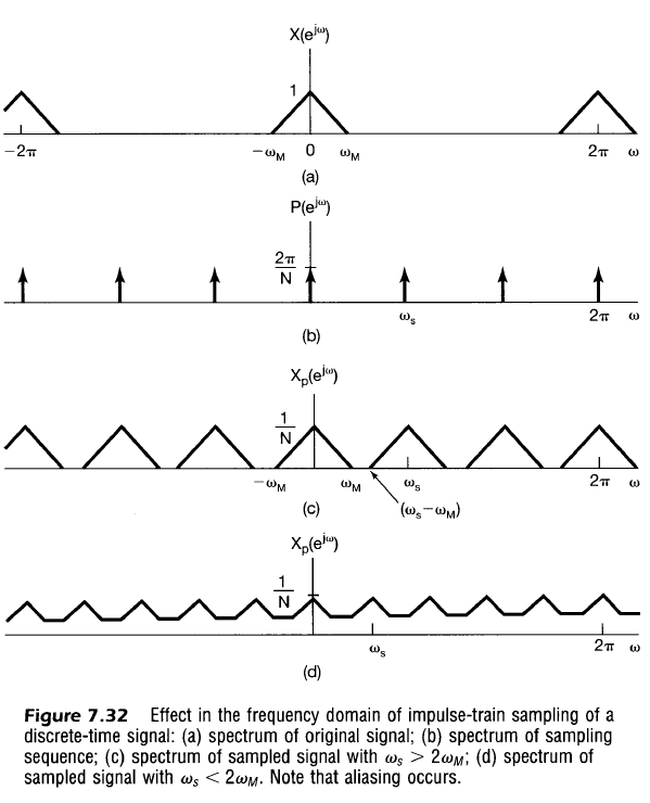
Note in the above graphs you can see that $X_p$ is replicated $N$ times on the interval $\omega \in [0, 2 \pi)$

Aliasing is avoided when

$$
\begin{align}
\omega_M &< \omega_s/2 \\
\omega_M &< \pi / N \\
N &< \pi / \omega_M \\
\end{align}
$$

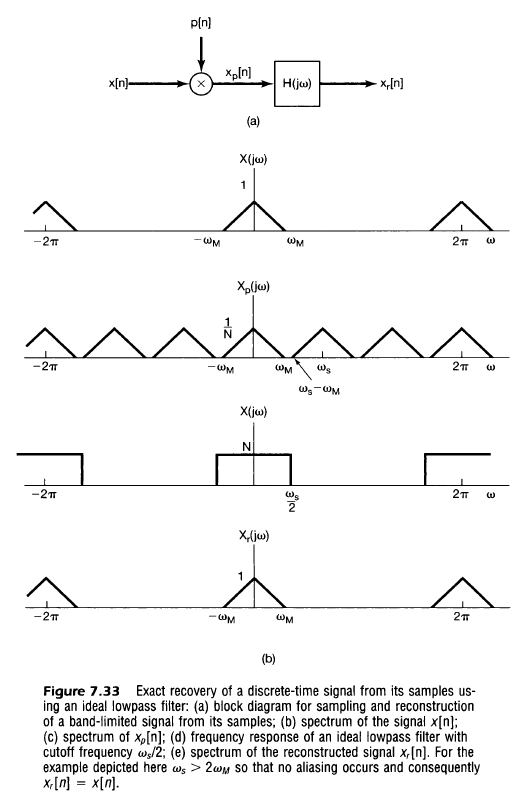
Note also that recovery can occur with an ideal lowpass filter

Downsampling (Decimation) and Upsampling

Called decimation to represent reducing samples by factor of 10.
$$
\begin{align}
x_b[n] &= x_p[nN] \\
x_b[n] &= x[nN] \\
\\
X_b(e^{j \omega}) &= \sum_{k=-\infty}^{\infty} x_b[k] e^{-j \omega k} \\
X_b(e^{j \omega}) &= \sum_{k=-\infty}^{\infty} x_p[kN] e^{-j \omega k} \\
\end{align}
$$

Using a new variable $n$ that is multiple integers of $N$, $n = kN$ and $k = n/N$ where

$$
\begin{align}

X_b(e^{j \omega}) &= \sum_{n \in { kN | k, N \in \mathbb{Z} }} x_p[n] e^{-j \omega n / N} \\

\end{align}
$$

and because all values of $x_p[k]$ are 0 outside of $n$ we can also say

$$
\begin{align}
X_b(e^{j \omega}) &= \sum_{n=-\infty}^{\infty} x_p[n] e^{-j \omega n / N} \\
X_b(e^{j \omega}) &= X_p \left( e^{j \omega / N} \right) \\
\end{align}
$$

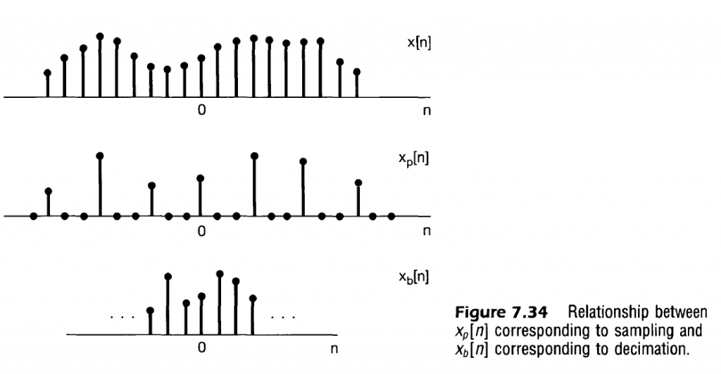
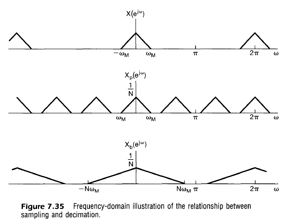
Note that $X_b$ is effectively a stretched out version of $X_p$. This makes sense intuitively as decimation/downsampling is effectively sampling the signal at a lower sampling rate.

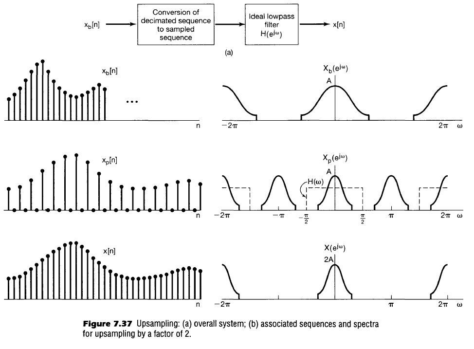
Upsampling may also be employed using a lowpass filter to convert to a higher equivalent sampling rate. This process is effctively the reverse of downsampling and is shown below.