A more rigorous description of this analysis is available on the Discrete Transforms page, but the continuous time analysis is done on this page for reference.
Intent
We previously found the key conceptualization that an input signal $x(t)$ into an LTI system yields an output $y(t)$ that is essentially a sum of impulse responses $h(t)$ that are scaled and time shifted by each location in $t$. This operation is called convolution and is represented by
$$
\begin{align}
x(t) &\rightarrow y(t) = x(t) * h(t) \\
x(t) &\rightarrow y(t) = \int_{-\infty}^{\infty} x(\tau) h(t-\tau) d\tau \\
\end{align}
$$
In the special case where the input signal is a sinusoid with a complex exponent, we have
$$
\begin{align}
x(t) &= e^{st} &&&s \in \mathbb{C} \\
\\
y(t) &= x(t) * h(t) \\
y(t) &= h(t) * x(t) \\
y(t) &= \int_{-\infty}^{\infty} h(\tau) x(t-\tau) d\tau \\
y(t) &= \int_{-\infty}^{\infty} h(\tau) e^{s(t-\tau)} d\tau \\
y(t) &= \int_{-\infty}^{\infty} h(\tau) e^{s(t-\tau)} d\tau \\
y(t) &= \int_{-\infty}^{\infty} h(\tau) e^{st} e^{-s\tau} d\tau \\
y(t) &= e^{st} \int_{-\infty}^{\infty} h(\tau) e^{-s\tau} d\tau \\
y(t) &= x(t) \int_{-\infty}^{\infty} h(\tau) e^{-s\tau} d\tau \\
\end{align}
$$
where we find the convenient result that the output is merely a scaled version of the input. It is then said that the eigenfunction is $e^{st}$ and the scaled output is the eigenvalue $H(s)$ for a specific $s$ where
$$
\begin{align}
H(s) &= \int_{-\infty}^{\infty} h(\tau) e^{-s\tau} d\tau \\
\end{align}
$$
Because LTI systems are linear, it is therefore desirable to express any input signal as a sum of complex exponentials, so it is easier to conceptualize the output as scaled versions of those sinusoids.
$$
\begin{align}
x(t) = e^{st} &\rightarrow y(t) = H(s) e^{st} \\
x(t) = \sum_q a_q e^{s_q t} &\rightarrow y(t) = \sum_q a_q H(s_q) e^{s_q t} \\
\end{align}
$$
The transforms explored below allow us to make this leap so that any signal may be represented as a sum of complex exponentials.
Continuous Time Fourier Series
Let’s say we have some signal $x(t)$ that is periodic with some fundamental period $T_0$. The Fourier Series is built on the assumption that this periodic signal can be represented as an infinite series of complex harmonics of fundamental frequency $\omega_0 = 2 \pi / T_0$
$$
\begin{align}
x(t) &= \sum_{k=-\infty}^{\infty} a_k e^{j k \omega_0 t} \\
\end{align}
$$
Now, the goal is to find what $a_k$s are needed to represent the original signal as a sum of complex harmonics. This can be done by multiplying both sides by another complex exponential and integrating over one period.
$$
\begin{align}
x(t) e^{-j q \omega_0 t} &= \sum_{k=-\infty}^{\infty} a_k e^{j k \omega_0 t} e^{-j q \omega_0 t} \\
\int_{T_0} x(t) e^{-j q \omega_0 t} dt &= \int_{T_0} \sum_{k=-\infty}^{\infty} a_k e^{j k \omega_0 t} e^{-j q \omega_0 t} dt \\
\int_{T_0} x(t) e^{-j q \omega_0 t} dt &= \int_{T_0} \sum_{k=-\infty}^{\infty} a_k e^{j (k – q) \omega_0 t} dt \\
\int_{T_0} x(t) e^{-j q \omega_0 t} dt &= \sum_{k=-\infty}^{\infty} a_k \left[ \int_{T_0} e^{j (k – q) \omega_0 t} dt \right] \\
\end{align}
$$
Looking at the integral on the RHS, note that harmonics are defined with $k \in \mathbb{Z}$. If we restrict our operations such that $k-q \in \mathbb{Z} \implies q \in \mathbb{Z}$ we note that
$$
\forall k, q \in \mathbb{Z}, \int_{T_0} e^{j (k – q) \omega_0 t} dt = \cases{
\begin{align}
T_0 &&&k = q \\
0 &&&k \neq q \\
\end{align}
}
$$
In other words, if we know that the LHS is nonzero, then we must have $k=q$ in which case
$$
\begin{align}
\int_{T_0} x(t) e^{-j q \omega_0 t} dt &= \sum_{k=q} a_k \left[ \int_{T_0} 1 dt \right] &&&(k=q) \land (k,q \in \mathbb{Z}) \\
\int_{T_0} x(t) e^{-j q \omega_0 t} dt &= a_q T_0 &&&(k=q) \land (k,q \in \mathbb{Z}) \\
a_q &= \frac{1}{T_0} \int_{T_0} x(t) e^{-j q \omega_0 t} dt &&&(k=q) \land (k,q \in \mathbb{Z}) \\
\end{align}
$$
Replacing $q$ with $k$ for notation consistency, we have the synthesis and analysis equations
$$
\boxed{
\begin{align}
x(t) &= \sum_{k=-\infty}^{\infty} a_k e^{j k \omega_0 t} \\
a_k &= \frac{1}{T_0} \int_{T_0} x(t) e^{-j k \omega_0 t} dt \\
\end{align}
}
$$
Continuous Time Fourier Transform
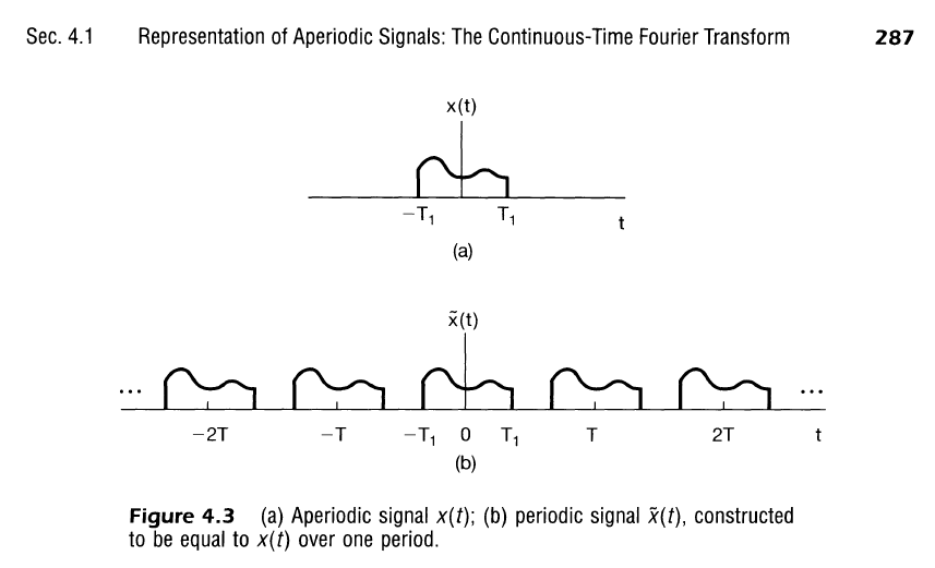
The Fourier series assumes we are working with periodic signals. However, this approach can be extended to aperiodic signals with some careful manipulation.
Assume we have a periodic signal with a Fourier Series representation such that
$$
\begin{align}
\tilde{x}(t) &= \sum_{k=-\infty}^{\infty} a_k e^{j k \omega_0 t} \\
\end{align}
$$
From the Fourier Series
$$
\tilde{x}(t) = \sum_{k=-\infty}^{\infty} a_k e^{j k \omega_0 t} \stackrel{FS}{\leftrightarrow} a_k = \frac{1}{T_0} \int_{T} \tilde{x}(t) e^{-j k \omega_0 t} dt
$$
Now assume we define an aperiodic signal $x(t)$ that is the same as $\tilde{x}(t)$ over one period, and 0 otherwise. That is
$$
x(t) = \cases{
\begin{align}
\tilde{x}(t) &&&t \in [t_1, t_2] &&t_2 – t_1 = T_0 \\
0 &&&\text{Otherwise} \\
\end{align}
}
$$
Note also that
$$
\begin{align}
a_k &= \frac{1}{T_0} \int_{T_0} \tilde{x}(t) e^{-j k \omega_0 t} dt \\
a_k &= \frac{1}{T_0} \int_{T_0} x(t) e^{-j k \omega_0 t} dt \\
a_k &= \frac{1}{T_0} \int_{-\infty}^{\infty} x(t) e^{-j k \omega_0 t} dt \\
\end{align}
$$
because to determine $a_k$ we are only concerned with one period of the signal and $x(t)$ is 0 everywhere outside that period. We next define the Envelope Function $X(s)$ as a function of the aperiodic signal $x(t)$
$$
X(s) = \int_{-\infty}^{\infty} x(t) e^{-s t} dt \\
$$
so now the Fourier Series coefficents can be rewritten as
$$
\begin{align}
a_k &= \frac{1}{T_0} X(j k \omega_0) \\
\end{align}
$$
and the synthesis equation for the periodic signal becomes
$$
\begin{align}
\tilde{x}(t) &= \sum_{k=-\infty}^{\infty} \frac{1}{T_0} X(j k \omega_0) e^{j k \omega_0 t} \\
\tilde{x}(t) &= \sum_{k=-\infty}^{\infty} \frac{\omega_0}{2 \pi} X(j k \omega_0) e^{j k \omega_0 t} \\
\tilde{x}(t) &= \frac{1}{2 \pi} \sum_{k=-\infty}^{\infty} X(j k \omega_0) e^{j k \omega_0 t} \omega_0 \\
\end{align}
$$
Now consider a new periodic signal $\tilde{x}_1(t)$ that is the same as $\tilde{x}(t)$ over some $T_0$, but this new signal repeats some $T > T_0$. To accommodate this new longer period (decreased frequency) time is added to each period where $\tilde{x}_1(t) = 0$. In this case, we are essentially expanding the period of $\tilde{x}(t)$ until it resembles $x(t)$. As $T \rightarrow \infty$ we may observe the following phenomena
$$
\begin{align}
\omega_0 \rightarrow d \omega \\
k \omega_0 \rightarrow \omega \\
\tilde{x} \rightarrow x \\
\end{align}
$$
So that the Analysis and Synthesis equation become, for any signal,
$$
\boxed{
\begin{align}
x(t) &= \frac{1}{2 \pi}\int_{-\infty}^{\infty} X(j \omega) e^{j \omega t} d \omega \\
X(j \omega) &= \int_{-\infty}^{\infty} x(t) e^{-j \omega t} dt \\
\end{align}
}
$$
Note that $X$ is a function of $\omega$. In summary, these equations suggest that
- Any continuous signal (periodic or aperiodic) may be represented by a summation of complex exponentials in the frequency domain $\omega$
- The amplitude of a signal’s constituent complex exponentials are described by the function $\frac{1}{2 \pi} X(j \omega)$ which may, itself, be complex.
- The Fourier Series coefficients of a continuous periodic signal with fundamental period $T_0$ and fundamental frequency $\omega_0$ may be determined from the Envelope function used in the Fourier Transform as
$$
\begin{align}
a_k = \frac{1}{T_0} X(j k \omega_0) &&k \in \mathbb{Z} \\
\end{align}
$$
Laplace Transform
Note that for the Continuous Fourier Transform, we have been using the analysis function defined by
$$
X(j \omega)
$$
where $j \omega$ is completely imaginary. However, we may further generalize the independent variable of this function to accept any complex input (any location in the complex plane). In this way, we modify our original starting point and assume that a signal can be represented as an infinite sum of complex exponentials with harmonic frequency components.
$$
\begin{align}
\tilde{x}(t) &= \sum_{k=-\infty}^{\infty} a_k e^{(\sigma + j k \omega_0) t} \\
\end{align}
$$
The coefficients, $a_k$ are then determined.
$$
\begin{align}
\tilde{x}(t) &= \sum_{k=-\infty}^{\infty} a_k e^{(\sigma + j k \omega_0) t} \\
\int_{T_0} \tilde{x}(t) e^{-(\sigma + j q \omega_0) t} dt &= \int_{T_0} \sum_{k=-\infty}^{\infty} a_k e^{(\sigma + j k \omega_0) t} e^{-(\sigma + j q \omega_0) t} dt \\
\int_{T_0} \tilde{x}(t) e^{-(\sigma + j q \omega_0) t} dt &= \int_{T_0} \sum_{k=-\infty}^{\infty} a_k e^{\sigma t -\sigma t} e^{j (k – q) \omega_0 t} dt \\
\int_{T_0} \tilde{x}(t) e^{-(\sigma + j q \omega_0) t} dt &= \sum_{k=-\infty}^{\infty} a_k \left[ \int_{T_0} e^{j (k – q) \omega_0 t} dt \right] \\
\end{align}
$$
We effectively get the same implication as before: for the kth harmonic, $k, q \in \mathbb{Z} \implies$
$$
\forall k, q \in \mathbb{Z}, \int_{T_0} e^{j (k – q) \omega_0 t} dt = \cases{
\begin{align}
T_0 &&&k = q \\
0 &&&k \neq q \\
\end{align}
}
$$
Assuming the LHS is nonzero, we can say $k=q$, $k,q \in \mathbb{Z} \implies $
$$
\begin{align}
\int_{T_0} \tilde{x}(t) e^{-(\sigma + j q \omega_0) t} dt &= a_q T_0 \\
a_q &= \frac{1}{T_0} \int_{T_0} \tilde{x}(t) e^{-(\sigma + j q \omega_0) t} dt \\
a_k &= \frac{1}{T_0} \int_{T_0} \tilde{x}(t) e^{-(\sigma + j q \omega_0) t} dt \\
\end{align}
$$
Now consider a new finite duration signal $x(t)$ where
$$
\begin{align}
t_2 – t_1 = T_0 \\
\\
\forall t \in [t_1, t_2], x(t) = \tilde{x}(t) \\
\end{align}
$$
then we can expand the region of integration such that the following statements are also true.
$$
\begin{align}
a_k &= \frac{1}{T_0} \int_{T_0} x(t) e^{-(\sigma + j k \omega_0) t} dt \\
a_k &= \frac{1}{T_0} \int_{-\infty}^{\infty} x(t) e^{-(\sigma + j k \omega_0) t} dt \\
\end{align}
$$
Now we define the envelope function
$$
X(\sigma + j k \omega_0) = \int_{-\infty}^{\infty} x(t) e^{-(\sigma + j k \omega_0) t} dt \\
$$
the Fourier Series coefficients then can be rewritten as
$$
\begin{align}
a_k &= \frac{1}{T_0} X(\sigma + j k \omega_0) \\
\end{align}
$$
and the synthesis equation for the periodic signal becomes
$$
\begin{align}
\tilde{x}(t) &= \sum_{k=-\infty}^{\infty} \left[ \frac{1}{T_0} X(\sigma + j k \omega_0) \right] e^{(\sigma + j k \omega_0) t} \\
\tilde{x}(t) &= \sum_{k=-\infty}^{\infty} \frac{\omega_0}{2 \pi} X(\sigma + j k \omega_0) e^{(\sigma + j k \omega_0) t} \\
\tilde{x}(t) &= \frac{1}{2 \pi} \sum_{k=-\infty}^{\infty} X(\sigma + j k \omega_0) e^{(\sigma + j k \omega_0) t} \omega_0 \\
\\
\omega_0 &\rightarrow d \omega \\
k \omega_0 &\rightarrow \omega \\
\tilde{x} &\rightarrow x \\
\end{align}
$$
$$
\begin{align}
x(t) &= \frac{1}{2 \pi} \int_{-\infty}^{\infty} X(\sigma + j \omega) e^{(\sigma + j \omega) t} d \omega \\
X(\sigma + j \omega) &= \int_{-\infty}^{\infty} x(t) e^{-(\sigma + j \omega) t} dt
\end{align}
$$
The complex exponent is commonly simplified to use the variable $s = \sigma + j \omega$ giving the Synthesis and Analysis equations for the Laplace Transform
$$
\boxed{
\begin{align}
x(t) &= \frac{1}{2 \pi} \int_{-\infty}^{\infty} X(s) e^{st} d \omega \\
X(s) &= \int_{-\infty}^{\infty} x(t) e^{-st} dt
\end{align}
}
$$
To visualize this result in the complex plane, the Laplace Transform states that we can reconstruct a signal by integrating the envelope function $X(s)$ along a vertical line of constant $\sigma$ assuming that the integral converges. In the special case of the Fourier Transform, $\sigma = 0$ and this line cuts through the origin.
Note that we have an extra condition for the Laplace Transform that did not exist for the previous transforms: we must choose $s$ such that the integral converges. The set of $s$ that do converge is defined as the Region of Convergence and must be defined for each transform.
Region of Convergence
ROC = Region of Convergence. Values of $s$ for which the integral in the Laplace Transform converges. This must be included as part of the Laplace Transform answer.
If the order of the numerator in $X(s)$ is $k$ less than the denominator, then there is said to be $k$ zeros “at infinity” i.e. as $s \to \infty$ the magnitude of the envelope function approaches 0. The same is true for poles if the order of the denominator is less than the numerator.
Properties
1. ROC consists of strips parallel to $j \omega$ axis. This is because the real part of $s$ is what determines if the integral converges
2. If $X(s)$ is rational, ROC does not contain any poles. $X(s)$ is infinite at a pole, so convergence is impossible
3. If $x(t)$ is finite duration and absolutely integrable, then ROC is the entire s-plane. An exponential multiplied by signal that is of finite duration is always bounded.
4. If $x(t)$ is right sided and if the line $Re\{s\} = \sigma_0$ is in the ROC (is vertical), then all values of $s$ such that $Re\{s\} > \sigma_0$ will also be in the ROC.
To prove this, consider that for a right sided signal where $\forall t < t_0, x(t) = 0$, we may rewrite the analysis equation as
$$
\begin{align}
X(s) &= \int_{-\infty}^{\infty} x(t) e^{-st} dt \\
X(s) &= \int_{t_0}^{\infty} x(t) e^{-st} dt \\
X(s) &= \int_{t_0}^{\infty} x(t) e^{-(\sigma + j \omega)t} dt \\
X(s) &= \int_{t_0}^{\infty} x(t) e^{-\sigma t} e^{j \omega t} dt \\
\end{align}
$$
Convergence of the integral is then determined solely by $x(t) e^{-st}$. Because the signal is absolutely integrable and bounded on one side by a finite number $t_0$, then divergence is only determined by the real part of the exponent, $\sigma$ as $t \to \infty$. If $\sigma_0$ converges, then $\forall \sigma > \sigma_0$ the integral converges faster.
5. If $x(t)$ is left sided and if the line $Re\{s\} = \sigma_0$ is in the ROC (is vertical), then all values of $s$ such that $Re\{s\} < \sigma_0$ will also be in the ROC. Using the same logic as above, the analysis equation in this case becomes
$$
\begin{align}
X(s) &= \int_{-\infty}^{t_0} x(t) e^{-\sigma t} e^{j \omega t} dt \\
X(s) &= -\int_{t_0}^{-\infty} x(t) e^{-\sigma t} e^{-j \omega t} dt \\
\end{align}
$$
Assuming $x(t)$ is absolutely integrable, then we again look for when the integral diverges as $t \to -\infty$. Because the sign of the exponent with the real part is reversed, then if $\sigma_0$ converges, then $\forall \sigma < \sigma_0$ the integral would converge faster.
6. If $X(s)$ is rational then its ROC is bounded by poles or extends to infinity.
7. If $X(s)$ is rational, then $\text{Right-Sided } x(t) \implies \text{ROC is right of rightmost pole}$ and $\text{Left-Sided } x(t) \implies \text{ROC is left of leftmost pole}$. Causal systems have ROC that is right of rightmost pole or entire s-plane.
Stable, causal systems must have all poles to the left side of the $j \omega$-axis.